Description

Such a diagram (basically a graphical analog computation device) is called a nomogram. The linked Wikipedia article gives and excellent overview.

Python and PostScript

Although PostScript is good at creating graphics, I find it cumbersome for calculations. So in this case, I’m using Python to do most of the calculations and have it generate PostScript commands for drawing.

Generating the nomogram

In this example I’m using two vertical axes for the input parameters, which are the measured quantities for the gelcoat and peroxide. The major ticks are spaced 10 mm apart for convenience. It is not a requirement to use similar spaced axes, it isn’t even necessary to use linear axes. Depending on the formula of the problem it could be advantageous to use logarithmic scales for one or both axes.

The heart of the program are two variables that hold the x-coordinates of the input axes, and two functions that convert the values of the axes into y-coordinates

# Axis locations
xgel = 20  # mm
xper = 80  # mm


def ygel(g):
   """Calculates the y position for a given amount of gelcoat."""
   return 10 + (g - 600) * 1


def yper(p):
   """Calculates the y position for a given amount of peroxide."""
   return 100 + (p - 12) * -10  # mm

With this, we can draw the axes.

# Gelcoat axis with markings
print(f'{xgel} mm {ygel(600)} mm moveto {xgel} mm {ygel(700)} mm lineto stroke')
for k in range(600, 701):
   if k % 10 == 0:
      print(f'{xgel} mm {ygel(k)} mm moveto -5 mm 0 rlineto stroke')
      print(f'{xgel-10} mm {ygel(k)} mm moveto ({k}) align_center')
   elif k % 5 == 0:
      print(f'{xgel} mm {ygel(k)} mm moveto -2.5 mm 0 rlineto stroke')
   else:
      print('gsave')
      print('0.1 setlinewidth')
      print(f'{xgel} mm {ygel(k)} mm moveto -2 mm 0 rlineto stroke')
      print('grestore')

# Peroxide axis with markings
print(f'{xper} mm {yper(12)} mm moveto {xper} mm {yper(21)} mm lineto stroke')
for k in range(120, 211):
   kk = k / 10
   if k % 10 == 0:
      print(f'{xper} mm {yper(kk)} mm moveto 5 mm 0 rlineto stroke')
      print(f'{xper+10} mm {yper(kk)} mm moveto ({kk}) align_center')
   elif k % 5 == 0:
      print(f'{xper} mm {yper(kk)} mm moveto 2.5 mm 0 rlineto stroke')
   else:
      print('gsave')
      print('0.1 setlinewidth')
      print(f'{xper} mm {yper(kk)} mm moveto 2 mm 0 rlineto stroke')
      print('grestore')

The result (converted to PNG and scaled down) looks like the picture below.

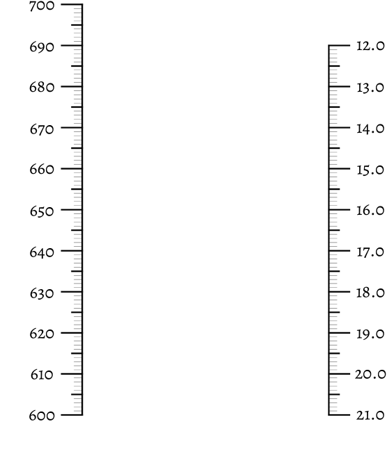
When printed (from the generated PDF), the major ticks are exactly 10 mm apart and the horizontal distance between the vertical axes is 60 mm. For this gelcoat, between 2% and 3% of peroxide is used. So the range on the right axis runs from 2% of 600 to 3% of 700.

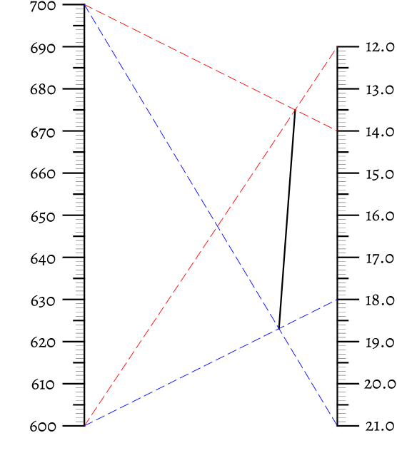
To draw the line that will have the ratio on it, we calculate 2% and 3% of 600 and 700 and draw the lines between those points on both axes. Their intersections define the limits of the axis for the ratios. The code for defining lines and calculating intersections is given below.

def line(p, q):
   """Create the line function passing through points P and Q.
   By solving py = a·px + b and qy = a·qx + b.

   Arguments:
      p: Point coordinates as a 2-tuple.
      q: Point coordinates as a 2-tuple.

   Returns:
      A 2-tuple (a, b) representing the line y = ax + b
   """
   (px, py), (qx, qy) = p, q
   dx, dy = px - qx, py - qy
   if dx == 0:
      raise ValueError('y is not a function of x')
   a = dy / dx
   b = py - a * px
   return (a, b)


def intersect(j, k):
   """Solve the intersection between two lines j and k.

   Arguments:
      j: 2-tuple (a, b) representing the line y = a·x + b.
      k: 2-tuple (c, d) representing the line y = c·x + d.

   Returns:
      The intersection point as a 2-tuple (x, y).
   """
   (a, b), (c, d) = j, k
   if a == c:
      raise ValueError('parallel lines')
   x = (d - b) / (a - c)
   y = a*x + b
   return (x, y)

This code speaks for itself. The result is shown below. The lines for 2% are in red, and those for 3% are in blue. This should also make clear why the scale on the right axis in inverted. If not, the ratio axis would not lie between the two input axes.

How do we know that the third axis is a line? Basically because the relation between gelcoat, peroxide and ratio is linear. And because I used the same intersection method to calculate the locations of all the tick marks on the ratio axis. When I plotted them they all ended up on the previously drawn line.

Note that this calculation method always works. Even if the third axis is not a straight line.

The code for drawing the tick marks on the ratio axis is given below.

# Calculate the angle for the ratio labels
p1 = (xgel, ygel(600))
p3 = (xgel, ygel(700))
p2 = (xper, yper(12))
p4 = (xper, yper(14))
# 2%
ln1 = line(p1, p2)
ln2 = line(p3, p4)
intersect2 = intersect(ln1, ln2)
# 3%
p5 = (xper, yper(18))
p6 = (xper, yper(21))
ln3 = line(p1, p5)
ln4 = line(p3, p6)
intersect3 = intersect(ln3, ln4)
print(
   f'{intersect2[0]} mm {intersect2[1]} mm moveto '
   f'{intersect3[0]} mm {intersect3[1]} mm lineto stroke'
)
dx = intersect2[0] - intersect3[0]
dy = intersect2[1] - intersect3[1]
dist = math.sqrt(dx * dx + dy * dy)
angle = math.degrees(math.atan2(dy, dx)) - 90

# ratio axis markings
for p in range(200, 301):
   pp = p / 100
   A, B = (xgel, ygel(600)), (xper, yper(pp / 100 * 600))
   C, D = (xgel, ygel(700)), (xper, yper(pp / 100 * 700))
   l1 = line(A, B)
   l2 = line(C, D)
   ip = intersect(l1, l2)
   print('gsave')
   print(f'{ip[0]} mm {ip[1]} mm translate')
   print(f'{angle} rotate')
   if p % 10 == 0:
      print('0 0 moveto -5 mm 0 lineto stroke')
      val = f'{pp:.1f}'.replace('.', ',')
      print(f'-10 mm 0 moveto ({val} %) align_center')
   elif p % 5 == 0:
      print('0 0 moveto -2.5 mm 0 lineto stroke')
   else:
      print('gsave')
      print('0.1 setlinewidth')
      print('0 0 moveto -2 mm 0 lineto stroke')
      print('grestore')
   print('grestore')

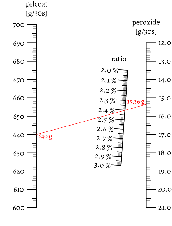
Finally we add the headings for the axes, and an example of how to read the nomogram. The result is shown below.

Creating PDF and PNG output

Both the PDF and PNG file are created from the Encapsulated PostScript generated by the python program.

To create tight-fitting PDF and PNG files, we need to know the bounding box of the generated PostScript code. This is done using ghostscript. Let’s look at some excerpts of the Makefile.

The fragment below specifies how to make an EPS file from a Python file. You should know that $< contains the name of the implied source (the Python file) and $@ represents the name of the output file.

.py.eps: Makefile
      python3 $< >body.ps
      echo '%!PS-Adobe-3.0 EPSF-3.0' >header.ps
      gs -q -sDEVICE=bbox -dBATCH -dNOPAUSE body.ps >>header.ps 2>&1
      cat header.ps body.ps > $@
      rm -f body.ps header.ps

First the Python code generates the body of the PostScript code. To make Encapsulated postscript, it has to have a header line and a BoundingBox. The header line is written to a file. Ghostscript is then used to calculate the bounding box for the body. This is then appended to the header. Finally, header and body are concatenated into the output file.

For converting the EPS file (now with BoundingBox) to PDF, ghostscript is used as well:

.eps.pdf:
      gs -q -sDEVICE=pdfwrite -dNOPAUSE -dBATCH -dEPSCrop \
      -sOutputFile=$@ -c .setpdfwrite -f $<

The EPSCrop flag is used to produce a PDF file the size of the extents of the EPS file instead of a whole page.

Producing a PNG file is slightly more complicated. To produce a fitting figure, you need to know the extents of the EPS figure, and then combine that with the desired resolution to get a suitable size of the image in pixels. That information is fed into Ghostscript.

Initially, I put this in the Makefile. But then I realized this could be useful elsewhere. So I rewrote it into a POSIX shell-script called eps2png.sh. You can find that in my scripts repository on Github. The relevant parts of it is shown below. Note that $f is the name of the input file.

OUTNAME=${f%.eps}.png
BB=`gs -q -sDEVICE=bbox -dBATCH -dNOPAUSE $f 2>&1 | grep %%BoundingBox`
WIDTH=`echo $BB | cut -d ' ' -f 4`
HEIGHT=`echo $BB | cut -d ' ' -f 5`
WPIX=$(($WIDTH*$RES/72))
HPIX=$(($HEIGHT*$RES/72))
gs -q -sDEVICE=${DEV} -dBATCH -dNOPAUSE -g${WPIX}x${HPIX} \
    -dTextAlphaBits=4 -dGraphicsAlphaBits=4 \
    -dFIXEDMEDIA -dPSFitPage -r${RES} -sOutputFile=${OUTNAME} $f

Note that WIDTH and HEIGHT are in PostScript points, i.e. 1/72 inch. Together with the resolution ($RES, defaulting to 300) in pixels per inch they are used to calculate the image extents in pixels, which are used in the -g option. It is also important to know that the arithmetic expressions in the shell are limited to integers. So division implicitly rounds the result to an integer! Hence we multiply first and divide as the last operation. Otherwise there would be significant rounding errors.