One way to look at how good encryption is to check how much the encrypted data lacks patterns (looks like random noise). An interesting way to check for patterns in a file is to convert it to a picture and look at it. I got the idea for this from the “spectra” software. The tool for converting data to images is ImageMagick. Additionally, making a histogram (counting the occurance of every possible byte value) and calculating the entropy is informative too.

First we look at a plain text file. I’m using a logfile. Since that is quite big, we isolate a portion using the dd command.

> dd if=procmail.log of=data.raw bs=1k count=1k
1024+0 records in
1024+0 records out
1048576 bytes transferred in 0.007041 secs (148924777 bytes/sec)

Next we use that data to make a set of two pictures. First, a black and white one (1 bit/pixel) from which we crop a block of 100×100 pixels from the left-top and enlarge it by a factor of three. Second a grayscale picture (8 bits/pixel) that is scaled to 300×300 pixels.

> convert -size 2896x2896 mono:data -crop 100x100+0+0 -scale 300x300 data-mono.png
> convert -size 1024x1024 -depth 8 gray:data -scale 300x300 data-gray.png

The -size argument for creating the monochrome pictures is the nearest integer to the square root of 1048576×8, which is also a multiple of 8.

Here is what the pictures looks like:

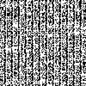
There are clear patterns visible in both images.

If you look closely at the left picture, there are vertical white stripes every eight pixels. The text is in ISO-8859 encoding, which is 8-bit but seldom has the eight bit set. (So to see these kinds of patters, it is a good idea to make the picture width a multiple of 8)

In the picture on the right, which shows the whole file, there are several things that strike the eye. There is a horizontal band of a distinctly different pattern in the top of the picture. There are several white stripes in the bottom of the picture, and there are dark patterns running from top to bottom.

The entropy of the data is 5.2120 bits/byte. This is calculated according to the definition of entropy in information theory:

255
-Σ  p(x)×log₂₅₆(p(x))
x=0

Where p(x) is the chance that a byte has the value x.

Next is the histogram.

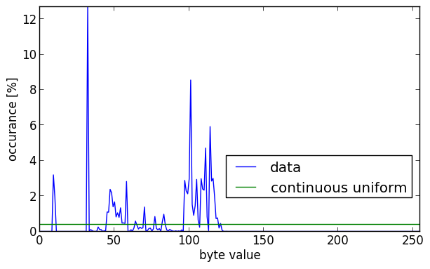
To interpret this picture you should know that in the ISO-8859 character set, the newline character has the integer value 10, the space 32 and the most common letter in English (‘e’) 101. This explains some of the high peaks in the histogram.

If this data was completely random, and if every value of a byte was equally probable (known as a continuous uniform distribution), all values would occur 1/256×100% = 0.390625% of the time. This is the green line in the histogram.

The following python program was used to generate the histograms and calculate entropy. It uses the excellent matplotlib library.

#!/usr/bin/env python

'''Make a histogram of the bytes in the input files, and calculate their
entropy.'''

import sys
import math
import subprocess
import matplotlib.pyplot as plt

def readdata(name):
    '''Read the data from a file and count how often each byte value
    occurs.'''
    f = open(name, 'rb')
    data = f.read()
    f.close()
    ba = bytearray(data)
    del data
    counts = [0]*256
    for b in ba:
        counts[b] += 1
    return (counts, float(len(ba)))

def entropy(counts, sz):
    '''Calculate the entropy of the data represented by the counts list'''
    ent = 0.0
    for b in counts:
        if b == 0:
            continue
        p = float(b)/sz
        ent -= p*math.log(p, 256)
    return ent*8

def histogram(counts, sz, name):
    '''Use matplotlib to create a histogram from the data'''
    xdata = [n for n in xrange(0, 256)]
    counts = [100*c/sz for c in counts]
    top = math.ceil(max(counts)*10.0)/10.0
    rnd = [1.0/256*100]*256
    fig = plt.figure(None, (7, 4), 100)
    plt.axis([0, 255, 0, top])
    plt.xlabel('byte value')
    plt.ylabel('occurance [%]')
    plt.plot(xdata, counts, label=name)
    plt.plot(xdata, rnd, label='continuous uniform')
    plt.legend(loc=(0.49, 0.15))
    plt.savefig('hist-' + name+'.png', bbox_inches='tight')
    plt.close()

if __name__ == '__main__':
    if len(sys.argv) < 2:
        sys.exit(1)
    for fn in sys.argv[1:]:
        hdata, size = readdata(fn)
        e = entropy(hdata, size)
        print "entropy of {} is {:.4f} bits/byte".format(fn, e)
        histogram(hdata, size, fn)

What happens when we encrypt this file? As a test we will be using openssl with Blowfish and AES encryption. For both we will use a long, pseudo-random password, generated like this:

> openssl rand -base64 21
HDtWa0yeOfy0r19IXgQeVRQjrN6W
> openssl bf -in data -out data.bf -pass pass:HDtWa0yeOfy0r19IXgQeVRQjrN6W

Next we will convert it to pictures, exactly as the raw data above.

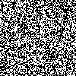
These look quite random to the naked eye, doesn’t it? The same goes for the histogram for the Blowfish encrypted data.

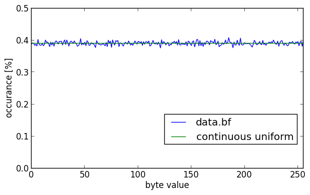
The graph looks nicely centered around the horizontal green line that indicates pure randomness with a continuous uniform distribution. It has a calculated entropy of 7.9998 bits/byte.

Next we encrypt the same data with AES.

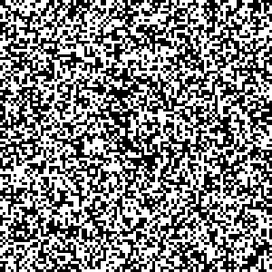
Both the 1 bit/pixel and 8 bits/pixel images look pretty random again, without obvious patterns. The histogram for the AES encrypted data looks almost the same as that of the Blowfish encrypted data. The entropy in this case is also 7.9998 bits/byte.

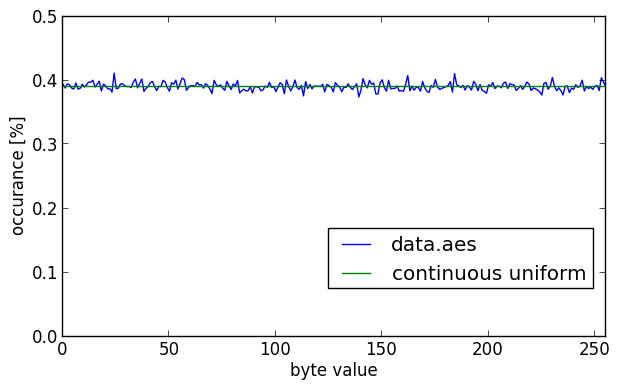
Two different and relatively modern encryption algorithms, used with a strong and salted key produce output that looks quite random.

So, for comparison we look at the output of FreeBSD’s pseudo-random number generator. This uses the Yarrow algorithm and gathers entropy from lan traffic and hardware interrupts:

> dd if=/dev/random of=random bs=1k count=1k
1024+0 records in
1024+0 records out
1048576 bytes transferred in 0.025319 secs (41414817 bytes/sec)
> convert -size 2896x2896 mono:random -crop 100x100+0+0 -scale 300x300 random-mono.png
> convert -size 1024x1024 -depth 8 gray:random -scale 300x300 random-gray.png

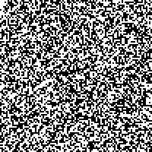
The histogram for the pseudo-random data:

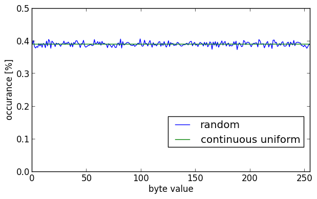
Again the calculated entropy is 7.9998 bits/byte. Both the encrypted and random data look pretty much the same in their grayscale images and their histograms. So it looks like algorithms like Blowfish and AES are pretty good. There are no discernable pattern in the data, and the histograms are pretty close to a continuous uniform distribution.

This illustrates that modern ciphers can be very resistent to known ciphertext attacks if:

• keys are long enough (and use a salt)
• algorithms were carefully researched (preferably in the open)
• the operator doesn’t make mistakes.
• procedures aren’t flawed