Recently I was listening to an MP3 file of a talk about no-till gardening when I noticed that there was a noticable buzz in the sound. I figured I would try my hand at sound filtering with Python as a learning experience.

The Python standard library doesn’t have a module for reading mp3 files, but it can handle wav files. So I used the mpg123 program to convert the file;

mpg123 -w 20130509talk.wav 20130509talk.mp3

This is quite a big file, so I also extracted a somewhat smaller file for testing;

mpg123 -k 7000 -n 2400 -w input.wav 20130509talk.mp3

The interesting portion of this uncompressed stereo wav file is basically a list of 16-bit integers with the left and right channel interspersed. So let us see first how we read data from a wav file and split the values for the channels. All this is done using Python version 2.7, but 3.3 should work as well.

import wave
import numpy as np
import matplotlib.pyplot as plt

wr = wave.open('input.wav', 'r')
sz = 44100 # Read and process 1 second at a time.
da = np.fromstring(wr.readframes(sz), dtype=np.int16)
left, right = da[0::2], da[1::2]

The first three lines are for importing the modules that we need for this code to work. The wave module is part of the standard library that comes with Python. The numpy (short for “numerical Python”) and matplotlib modules have to be installed seperately.

The wave.open() function opens the sound file for reading in this case. In this case the sound was sampled at 44.1 kHz. This is called the frame rate. I choose to analyse the sound in one second chunk for reasons that I’ll go into later. The readframes() method reads from the sound file and returns the data as a string. The fromstring() function from the numpy library converts the binary string into an array of 16 bit integers. The last line splits the array into the left and right channel arrays.

One of the standard ways to analyze sound is to look at the frequencies that are present in a sample. The standard way of doing that is with a discrete Fourier transform using the fast Fourier transform or FFT algorithm. What these basically in this case is to take a sound signal isolate the frequencies of sine waves that make up that sound.

So we are going to use the np.fft.rfft() function. This is meant for data that doesn’t contain complex numbers but just real numbers.

lf, rf = np.fft.rfft(left), np.fft.rfft(right)

The function np.fft.rfft() returns 1/2+1 as many numbers as it was given. This is because of the inherent symmetry in the transform. If the array were just as long as the input, the second half would be a mirror image of the first half.

Here I want to introduce the concept of the frequency resolution of FFT. Basically, this is the interval between the frequencies returned by the FFT. It is calculated by dividing the sampling frequency Fs by the number of samples n. Since the wav-file is sampled at 44100 Hz, and we take 44100 samples, the frequency resolution will be a convenient 1 Hz.

So for a sample of 44100 sounds, we get the intensity of the frequency from 0 to 22050 Hz. Which not accidentally covers the whole range that humans can hear. Let’s plot a figure of the sound and the frequencies of the left channel:

import matplotlib.pyplot as plt

plt.figure(1)
a = plt.subplot(211)
r = 2**16/2
a.set_ylim([-r, r])
a.set_xlabel('time [s]')
a.set_ylabel('sample value [-]')
x = np.arange(44100)/44100
plt.plot(x, left)
b = plt.subplot(212)
b.set_xscale('log')
b.set_xlabel('frequency [Hz]')
b.set_ylabel('|amplitude|')
plt.plot(abs(lf))
plt.savefig('sample-graph.png')

This figure is shown below.

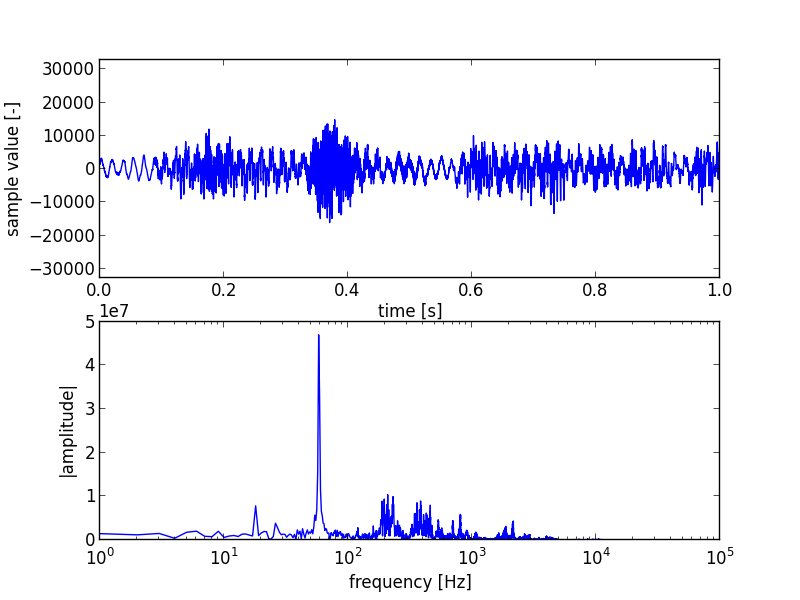
The top plot shows the typical combination of sine-wave structures of sound. But there is little there for us to see at first sight. The bottom plot is more interesting. It shows one big spike at and around 60 Hz. This is the frequency used for AC in the USA were the recording was made, and it was very noticable in the recording.

An AC circuit has two lines, power and neutral. Through damage in a wall or outlet the neutral wire can sometimes also carry a small amount of power. This reaches the microphone and is recorded. I made plots from several portions of the file, and this was the only big spike that was constantly there. When recording using the built-in microphone on a laptop a good way to prevent this is to disconnect the battery charger when recording.

The way to filter that sound is to set the amplitudes of the fft values around 60 Hz to 0, see (2) in the code below. In addition to filtering this peak, I’m also going to remove the frequencies below the human hearing range (1) and above the normal human voice range (3). Then we recreate the original signal via an inverse FFT (4).

highpass = 21 # Remove lower frequencies.
lowpass = 9000 # Remove higher frequencies.

lf[:highpass], rf[:highpass] = 0, 0 # high pass filter (1)
lf[55:66], rf[55:66] = 0, 0 # line noise filter (2)
lf[lowpass:], rf[lowpass:] = 0,0 # low pass filter (3)
nl, nr = np.fft.irfft(lf), np.fft.irfft(rf) # (4)
ns = np.column_stack((nl,nr)).ravel().astype(np.int16)

The last line combines the left and right channels again using the column_stack() function, interleaves the left and right samples using the ravel() method and finally converts them to 16-bit integers with the astype() method.

Plotting the changed sound and fft data again produces the figure below;

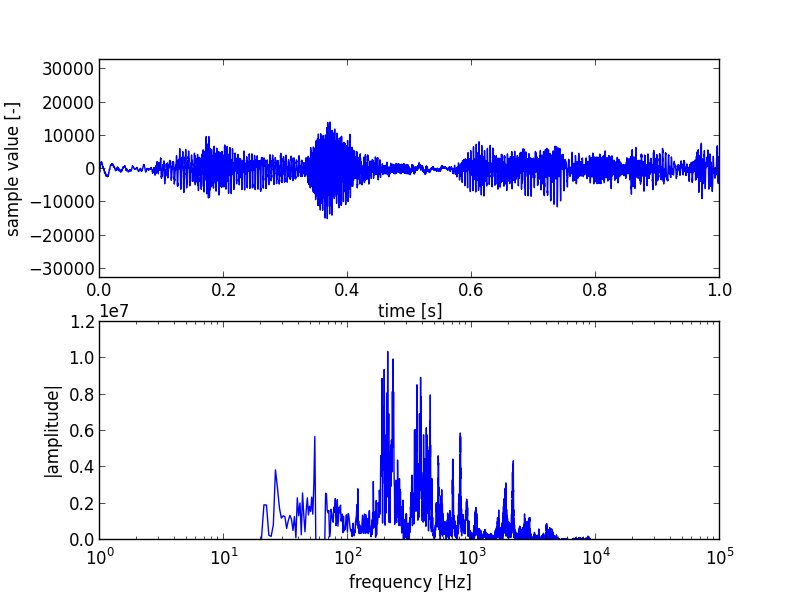
The big spike is now gone, as are the low and high tones. Looking back at the original and changed sound data, we can now see how the 60 Hz tone dominated the original sound data plot.

The resulting data can be converted to a string and written to a wav file again. This example was just for a one second sound sample. So to convert a complete file we have to loop over the whole contents. The complete program used to filter the complete file is given below;

import wave
import numpy as np
# compatibility with Python 3
from __future__ import print_function, division, unicode_literals

# Created input file with:
# mpg123  -w 20130509talk.wav 20130509talk.mp3
wr = wave.open('20130509talk.wav', 'r')
par = list(wr.getparams()) # Get the parameters from the input.
# This file is stereo, 2 bytes/sample, 44.1 kHz.
par[3] = 0 # The number of samples will be set by writeframes.

# Open the output file
ww = wave.open('filtered-talk.wav', 'w')
ww.setparams(tuple(par)) # Use the same parameters as the input file.

lowpass = 21 # Remove lower frequencies.
highpass = 9000 # Remove higher frequencies.

sz = wr.getframerate() # Read and process 1 second at a time.
c = int(wr.getnframes()/sz) # whole file
for num in range(c):
    print('Processing {}/{} s'.format(num+1, c))
    da = np.fromstring(wr.readframes(sz), dtype=np.int16)
    left, right = da[0::2], da[1::2] # left and right channel
    lf, rf = np.fft.rfft(left), np.fft.rfft(right)
    lf[:lowpass], rf[:lowpass] = 0, 0 # low pass filter
    lf[55:66], rf[55:66] = 0, 0 # line noise
    lf[highpass:], rf[highpass:] = 0,0 # high pass filter
    nl, nr = np.fft.irfft(lf), np.fft.irfft(rf)
    ns = np.column_stack((nl,nr)).ravel().astype(np.int16)
    ww.writeframes(ns.tostring())
# Close the files.
wr.close()
ww.close()

This technique works pretty well for these kind of disturbances, i.e. those that are very localized in the frequency domain.

During part of the talk there is a noticable sound or rushing air, which I suspect came from an airco unit or a laptop’s cooling fan. This gave no noticable single big spike. There were some smaller spikes but filtering those out wasn’t sufficient to eliminate them, probably because the sound was composed out of multiple harmonics. Additionally those spikes where in the frequency range of the normal spoken voice, so filtering them affected the talk too much.