What is a sandwich?

In structural engineering a sandwich is a composite structural element designed to withstand large bending loads relative to its light weight. Generally it consists of two relatively thin skins made of a stiff and strong material separated and connected by a light-weight core. This core can be e.g:

• polymer foam sheet,
• end-grain balsa wood,
• honeycomb sheet.

Additionally there is another light-weight construction in the form of discrete “stringer” plates set perpendicular between the skins. This is normally not considered a sandwich, though.

The stiff materials on the outside makes these elements structurally efficient at withstanding bending loads.

Why CalculiX?

Please note that this article is not an introduction into FEA for mechanical engineering! There are plenty of good books and free online resources for that. The book “Applied Mechanics of Solids” by Allan F. Bower is a good reference for solid mechanics. A web-version is available for free. It covers the principles of FEA for static linear elasticity in §7.2 and in more detail in §8.1.

CalculiX is an excellent free finite element software suite consisting of a pre- and post-processor called cgx and a solver called ccx. The capabilities of the solver compare favorably to much more expensive FEA software. But like all FEA software it has a pretty steep learning curve. Both the pre- and post-processor and the solver are programmed using a domain-specific language (“DSL”). Both of those are well documented in their respective manuals. The solver basically uses the same DSL as the commercial Abaqus FEA software.

For people new to CalculiX I would recommend the excellent repository of examples by professor Kraska.

Preprocessor

The CalculiX pre- and post-processor is called cgx. As a preprocessor it can be used to create 3D geometry and mesh it. It is not a 3D CAD-package, however. While it can be used to generate very complicated geometry (as witnessed by the small jet engine that can be found in the examples), this is not trivial.

Nevertheless I would still advocate using it wherever possible. The main reason is that it allows you to build completely parametric models that are trivial to change. This allows fast turnarounds for iterative design, which is for me one of the main use cases of mechanical FEA. It also creates structured meshes that produce excellent results.

If you want to analyze an existing geometry in the form of a STEP-file, I would recommend using gmsh to create a mesh and boundary conditions for the CalculiX solver.

Creating the geometry and mesh

In this example we will create a mesh where the elements representing different materials share nodes. This is the simplest way of generating such a mesh, but it has a significant disadvantage that we will cover later.

In general I would advise to use a simplified geometry for FEA. For example small holes and radii generally lead to a lot of small elements being necessary to model them correctly. This leads to very large meshes and thus a longer time necessary to solve the problem. In most cases their influence on the solution is small.

FEA software generally doesn’t care about which units you use, as long as they are consistent. In my FEA calculations I use SI units to avoid problems.

The example below is in the DSL for cgx. First we define the parameters that define the design.

# Dimensions
valu length 1.25
valu width 0.4
valu ttop 0.002
valu tbot 0.002
valu height 0.034

Here, ttop and tbot are the thicknesses of the top and bottom skins. The rest of the values should need no explanation.

When creating lines we have to give the number of “divisions” in those lines. These are basically hints for the mesh generator. Note that when using second order elements (more on that later) two divisions are needed for one element.

# Number of divisions for lines
valu ldiv 80
valu wdiv 18
valu hdiv 12
valu tdiv 6

So the product has 40 elements in its length, and 9 in its width. The core height has 6 elements in its thickness direction, and the skins 3. The reason for parametrizing these is that we want to be able to quickly find the minimum number of elements that gives a reliable answer. A standard strategy is to start with a low number of elements (for a fast calculation) and then keep increasing the number of elements until the found deformations and stresses stabilizes.

Lastly, we have some calculated values in the form of the core thickness.

valu t + ttop tbot
valu hc - height t

Here hc is the height of the core. The t intermediate is used because the valu command only allows calculations with one operator and two operands.

Next we get to actually generating the geometry. This follows a pattern that we see often in cgx examples.

• First we create a point.
• This is then swept into a line.
• The line is swept into a plane.
• The plane is swept into a solid.

The main reason for doing it this way (IMO) is to ensure that opposing edges have the same division counts and so can be automatically meshed without problems.

The swep command is a very powerful one. For example, the direction of the sweep is arbitrary and not necessarily perpendicular to the line or plane that is swept. Check the documentation for its different options.

Another thing to keep in mind is the use of sets. A set is basically a name for a collection of geometric entities, from solids back to points. We will use sets to later on assign different properties to different elements. First we create the bottom skin, encompassed in the set bot.

seto bot
    pnt ! 0 0 0
    swep bot new tra 0 width 0 wdiv  # creates a line
    swep bot new tra length 0 0 ldiv # creates a surface
    swep bot bot_t tra 0 0 tbot tdiv # creates a body
setc

Next, we create the core on top of the bottom skin.

seto core
    swep bot_t core_t tra 0 0 hc hdiv
setc

And finally the top skin.

seto top
    swep core_t top_t tra 0 0 ttop tdiv
setc

In this case top_t is the top surface of the sandwich we will use later.

Now comes the time to mesh the solid bodies. We will be using 20-node brick elements with reduced integration. This is a very well-behaved second-order element for these kinds of simulations. It has nodes on the corners of the brick, but also in the middle of the edges. See the CalculiX documentation for details. Note that the names of elements between cgx and ccx is not the same, which is somewhat confusing. In the pre-processor cgx this element is called “he20r”, while the solver ccx calls it “C3D20R”. Creating the mesh is now very simple.

elty all he20r
mesh all

(Note that “all” is a special set that contains all geometry.) Now that the elements are created, we need to define sets of nodes to apply loads and constraints. To define the constraint, we first create a set that only contains all nodes. Then we enquire which of those nodes are located at x=0.

seta nodes n all
enq nodes fix rec 0 _ _ 0.001 a

The set “fix” contains all the nodes at one end of the sandwich.

Now we need to save the nodes, elements and sets in a format that can be read by the solver.

send all abq
send bot abq nam
send core abq nam
send top abq nam
send fix abq nam

The first line creates a file called all.msh in which the nodes and elements are defined. Note that the set names are prefixed by a capital letter defining the art of the set. So the pre-processor set all is split into a set of all nodes called Nall and a set of elements called Eall.

The next the lines create node and element sets for the bottom skin, core and top skin respectively. They are called bot.nam, core.nam and top.nam. The element sets in those files (named Ebot, Ecore and Etop) are later used to assign different material properties to the elements.

We want to apply a distributed load to the top surface of the sandwich. Loads and constraints in FEA can actually only be applied to nodes, but the CalculiX solver will automatically convert a distributed load on a surface to loads on individual nodes in the surface.

Lastly, we export the surface to a file named top_t.sur.

send top_t abq sur

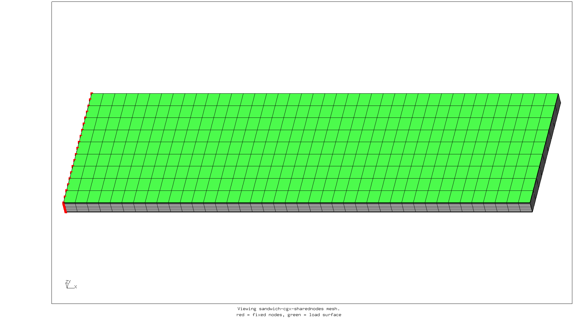
An image of the mesh is shown below. The colors indicate the nodes for fixation and the load surface.

Writing the analysis input file and running the analysis

Now that the mesh has been created, the analysis has to be defined in the DSL for the CalculiX solver ccx. The commands for this DSL are documented in the manual for ccx.

Comments in this file format start with ** in the first column. Commands start with a single *. The file starts with a heading, followed by a one-line description.

*HEADING
Clamped sandwich panel

Next we need to include the nodes, elements and sets defined in the pre-processor.

*INCLUDE, INPUT=all.msh
*INCLUDE, INPUT=bot.nam
*INCLUDE, INPUT=core.nam
*INCLUDE, INPUT=fix.nam
*INCLUDE, INPUT=top.nam
*INCLUDE, INPUT=top_t.sur

The nodes from the set fix.nam are used to fix the mesh in three directions.

*BOUNDARY
Nfix,1,3

Before we can assign materials to elements, we need to define them.

** Material properties skins
*MATERIAL, NAME=M_EN_AW_5754
*ELASTIC, TYPE=ISO
70e9,0.33,293
*DENSITY
2670

*MATERIAL, NAME=MS235J
*ELASTIC, TYPE=ISO
210e9,0.30,293
*DENSITY
7850

** Material properties core
*MATERIAL, NAME=MrohacellIG71
*ELASTIC,TYPE=ENGINEERING CONSTANTS
92e6,92e6,92e6,0.01,0.01,0.01,29e6,29e6
29e6,393
*DENSITY
75

In this case specifying the density is not strictly necessary. But I like to include it in case it is needed. Now we can assign the material to elements.

*SOLID SECTION, ELSET=Etop, MATERIAL=MS235J
*SOLID SECTION, ELSET=Ebot, MATERIAL=M_EN_AW_5754
*SOLID SECTION, ELSET=Ecore, MATERIAL=MrohacellIG71

In this case the top skin is made of structural steel and the bottom skin is made out of 5754 aluminium. Why? Basically because we can. The core material is Rohacell 71IG, a high-end foam that is often used in structural sandwich construction.

Finally, we need to define a calculation step. It is possible to define multiple calculation steps, but we will not do this now.

*STEP
*STATIC
** Loading 5 kN/m2 on top of top laminate.
*DLOAD
Stop_t,P5,5000
*NODE FILE
U,RF
*EL FILE
ZZS,ME
*END STEP

This is a calculation of the behavior of the sandwich under a static (constant) distributed load. For every node the displacement and reaction force is stored. For every element the stress and mechanical strain is stored.

On a UNIX-like system the solver is run as follows, assuming that the input file is named sandwich.inp.

/usr/bin/time -lh env OMP_NUM_THREADS=4 ccx -i sandwich
rm -f *.12d *.cvg *.sta *.log spooles.out

The time program is used to capture the time and memory used by the solver. The env command creates an environment variable that instruct the solver ccx to use the multithreaded spooles equation solver.

On my workstation (with Intel i7-7700 CPU) the solver run for this input takes around 7.5 seconds and has a maximum resident set size of approximately 1 GiB.

Viewing and assessing the results

To view the displacement, we run the post-processor as follows: cgx -b view-disp.fbd. The file view-disp.fbd contains the following commands for the post-processor.

read sandwich.frd

capt Viewing sandwich-cgx-sharednodes
ulin Z-displacement of sandwich panel
rot y
rot r 30
rot u 15
frame
zoom 0.8

cmap turbo
ds 1 e 3
view disp
view elem
scal d 10

The ds command determines what is displayed. Entity 3 of dataset 1 is usually the displacement in Z-direction.

The cgx display for the displacement looks like this:

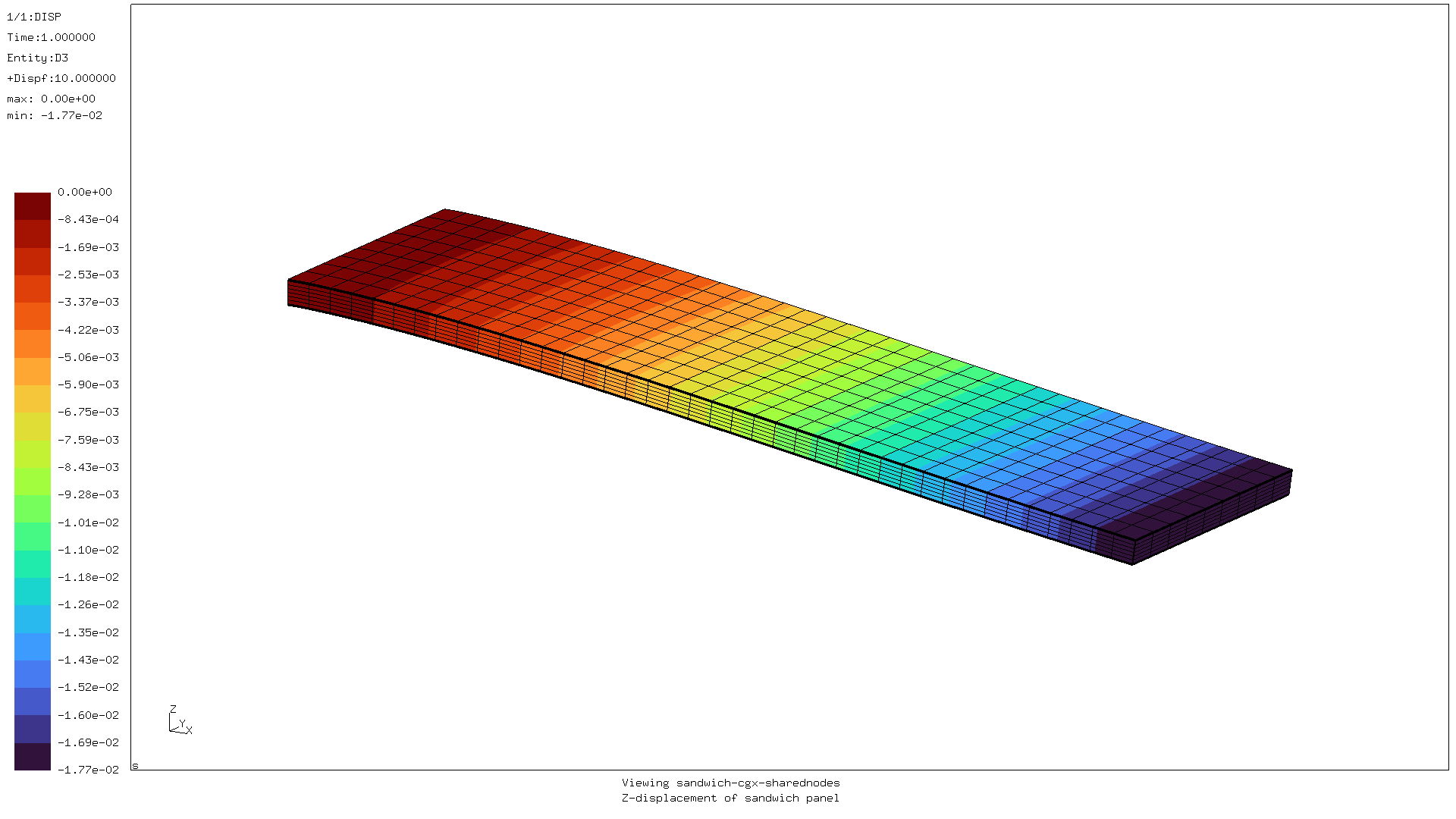
The deformed sandwich has the shape one would expect. The Z-deflection matches the value found when analysing this sandwich as a clamped beam (when shear is taken into account).

The global picture of the maximum principal stresses also looks OK:

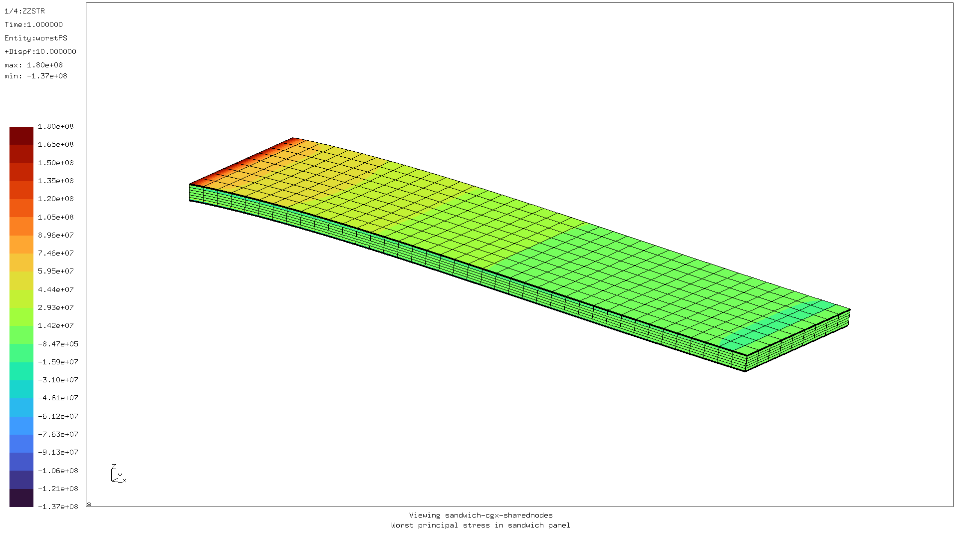
• On the free end, there is no stress.
• The stresses are highest at the clamped end.
• The stresses in the skins are much higher than those in the core, because the skins are much stiffer. Given the same deformation (on the interface between core and skins) the stress in the skin should be a lot higher.

However, when we switch to a detailed view of the von Mises stress near the clamped end, we see something odd:

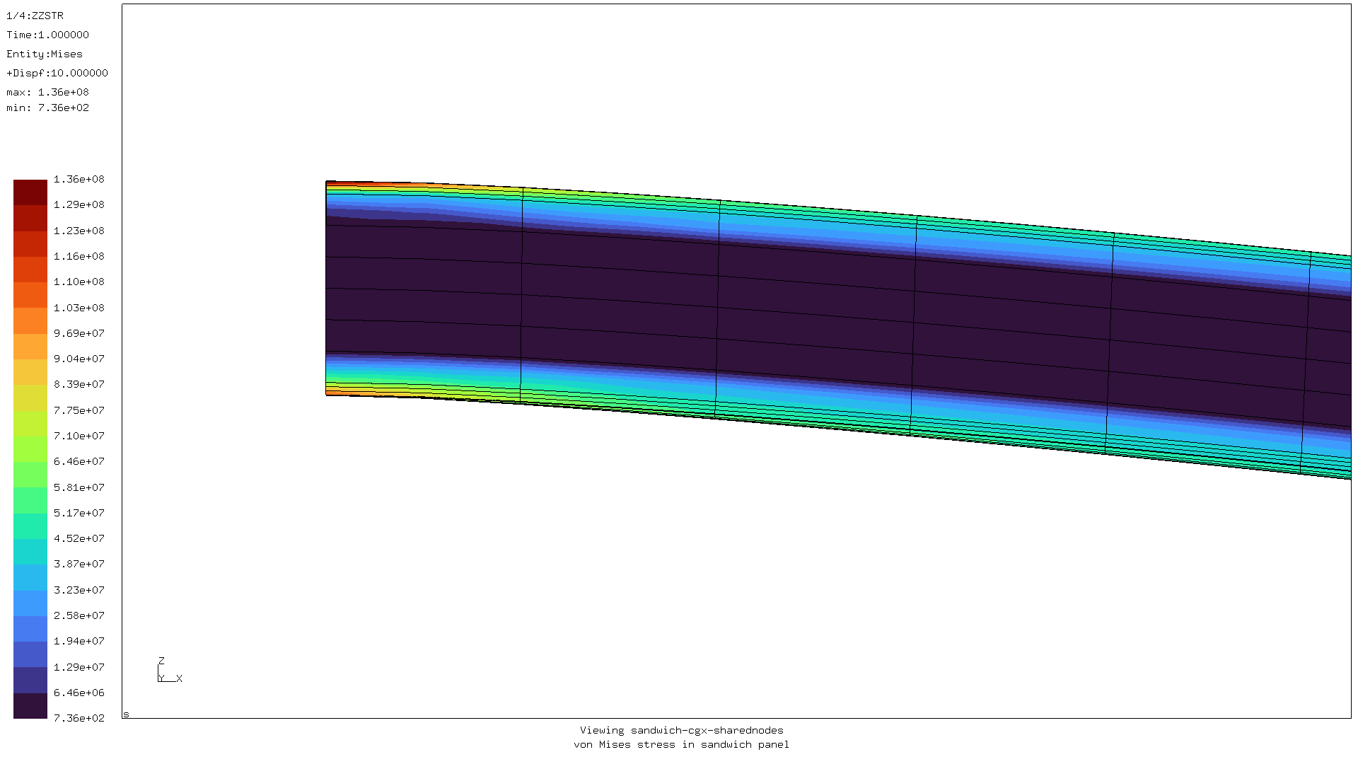
The stress from the skins “bleeds” into the core. Since the Young’s modulus of the skins is about three orders of magnitude larger than that of the core, this does not happen in reality.

Now it becomes important to understand how FEA works. Essentially, this method finds the displacement of the nodes based on the definition of the elements and the external loads. Based on these deformations, the stress in the integration points inside the elements are calculated. These are then extrapolated over the whole element and its nodes on the outsides. Finally, the values on the nodes from all adjacent elements are averaged.

It is this final averaging step that causes the problem in this case. To prevent that, we need to make sure that the skins and the cores do not share nodes. For a realistic result, they do have to be connected though. This can be accomplished using equations or *TIE-constraints. How this is done will be shown in a later article.