The nature of the problem

1. We want to prevent nodal averaging of stresses between element sets of different materials.
2. But when running the analysis we still want the different materials to be connected.

To satisfy the first requirement, we create the meshes such that the different bodies do not share nodes. This might lead to nodes from different element sets occupying the same position, but that it not necessarily a problem.

To meet the second requirement we are going to use the neigh command of the pre-processor to generate ties between close surfaces.

Mesh without shared node

The main difference is in how we create the sets for the different bodies. Instead of taking the top surface of the previous layer and extrude it, we copy it first.

As a reminder, this was the original code.

seto bot
    pnt ! 0 0 0
    swep bot new tra 0 width 0 wdiv  # creates a line
    swep bot new tra length 0 0 ldiv # creates a surface
    swep bot bot_t tra 0 0 tbot tdiv # creates a body
setc
seto core
    swep bot_t core_t tra 0 0 hc hdiv
setc
seto top
    swep core_t top_t tra 0 0 ttop tdiv
setc

Now we do it like this. Note that creating the set bot hasn’t changed.

seto bot
    pnt ! 0 0 0
    swep bot new tra 0 width 0 wdiv  # creates a line
    swep bot new tra length 0 0 ldiv # creates a surface
    swep bot bot_t tra 0 0 tbot tdiv # creates a body
setc
seto core
    copy bot_t core_b tra 0 0 0
    swep core_b core_t tra 0 0 hc hdiv
setc
seto top
    copy core_t top_b tra 0 0 0
    swep top_b top_t tra 0 0 ttop tdiv
setc

Generating and using ties

After creating the mesh, we use the neigh command with the tie option.

# Create mesh and write nodes and elements
elty all he20r
mesh all

# Create interlayer contact
neigh all 1e-5 abq tie

This neigh command will generate some files with the names DCF*.sur and ICF*.sur and a file neigh.con that will have to be included in the solver input file. Personally, I like to combine the surface files into a single file for convenience:

cat DCF* ICF* > ties.sur
rm ICF* DCF*

So we can include them to the solver command file sandwich.inp:

*INCLUDE, INPUT=neigh.con
*INCLUDE, INPUT=ties.sur

The rest of the solver command file can be retained unchanged.

Running the analysis and results

This has a cost in both runtime and memory consumption. The runtime goes from 7.5 seconds to 11.6 seconds. The maximum resident set size goes from 1 GiB to 1.3 GiB.

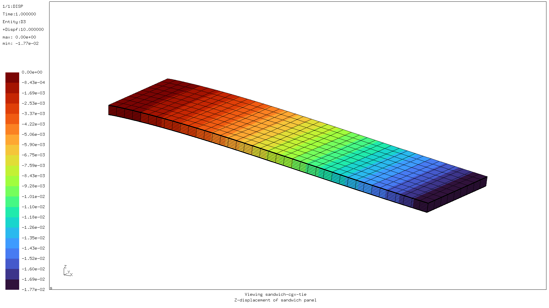
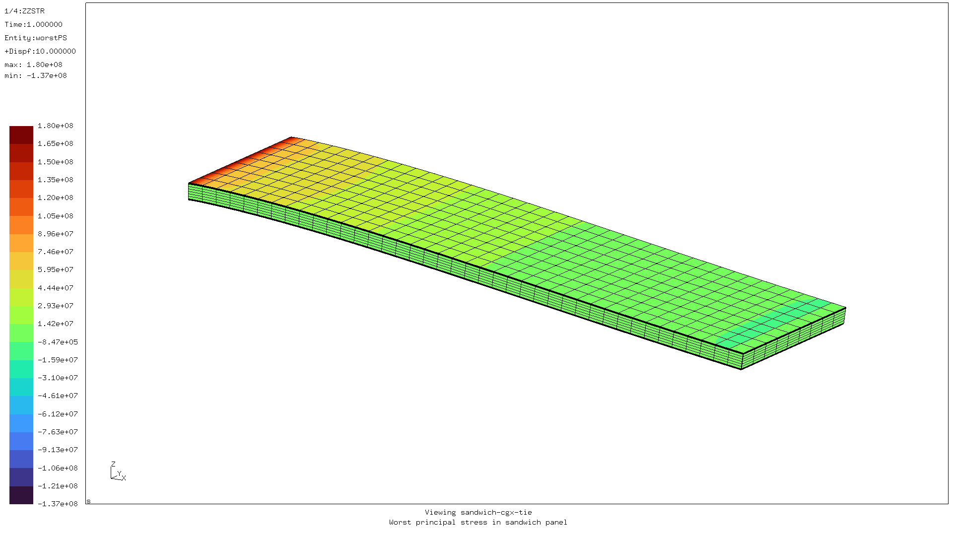
The global displacement and stress images don’t change:

But the stress bleed into the core is now gone:

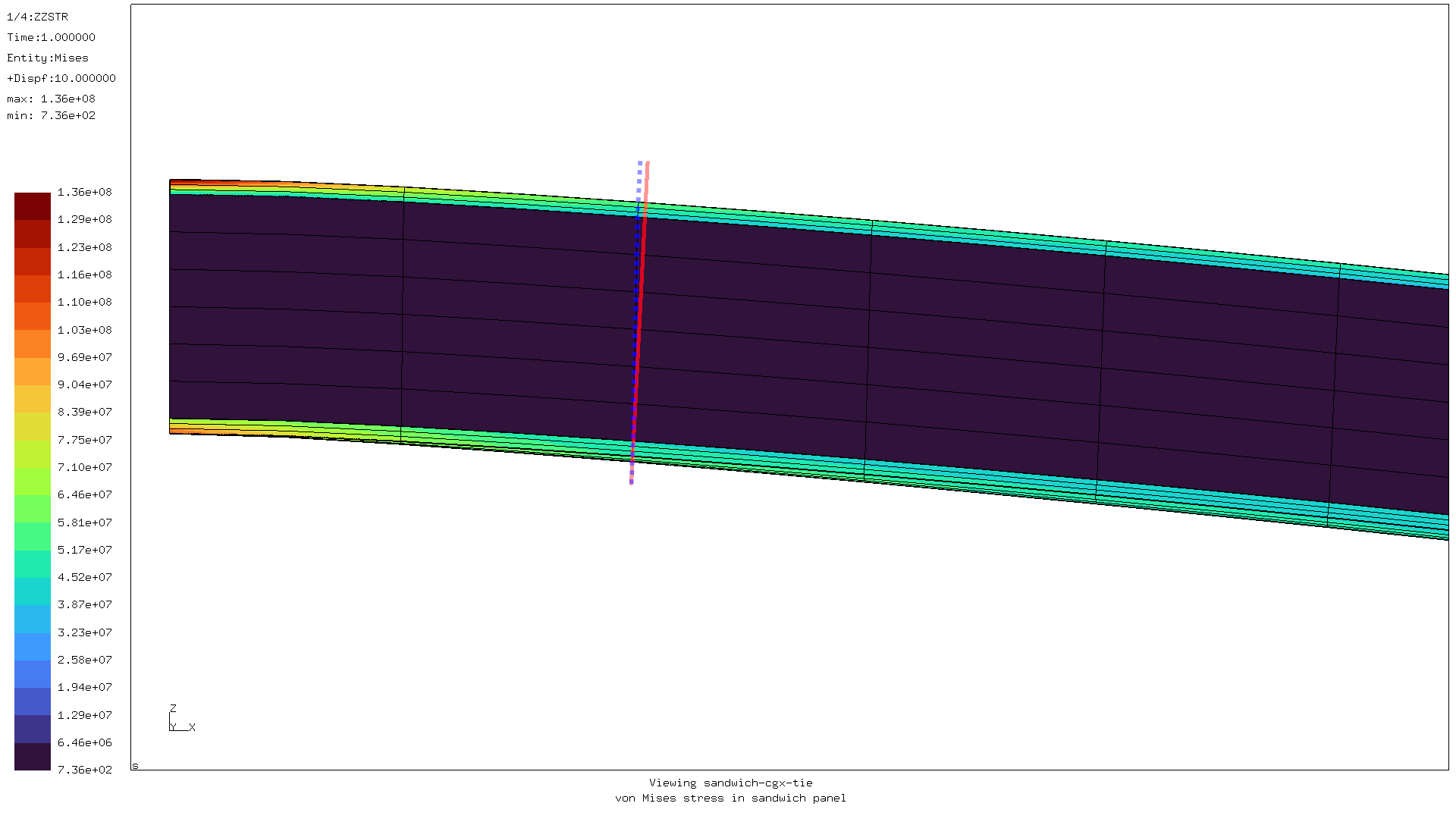
Because of the structured mesh you can also clearly see the effects of shear deformation in the core by looking at the vertical edges.

In a situation of pure bending (i.e. in a material with a very high shear modulus, where shear plays almost no role) one would expect the cross-section to be a straight line, perpendicular to top and bottom surface. Like the solid red line in the picture above.

Instead, the cross section of the bottom layer is shifted with respect to the top layer, as indicated by the blue dashed line.

In the picture below, the deflection over the sandwich panel calculated by different methods is compared.

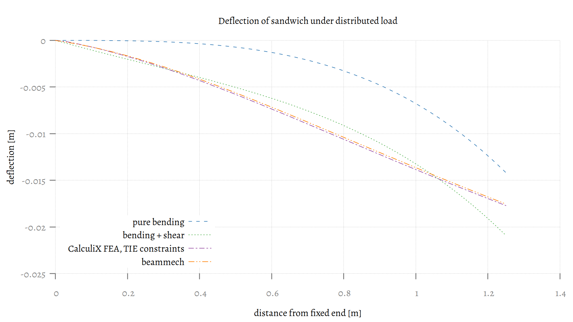
The dashed blue line representing pure bending is simply following the deflection formula that one can find in mechanics textbooks for a clamped beam of constant cross-section properties and with evenly distributed loading. The deflection at the free end is given by:

(This is derived by integration from the differential equation (d²y)/(dx²) = (M)/(E⋅I))

This severely under predicts the deflection in this case because it doesn’t take shear into account. For e.g. metal beams this is fine because the shear stiffness in that case is so high that shear deformation is not an issue. But for sandwich beams like this, it is definitely a problem.

One can integrate the differential equation for shear deformation (dy)/(dx) = (αD)/(G⋅A)). In this case that would yield y_B =  − (α⋅Q⋅L)/(2⋅G⋅A) for the shear deflection at the free end. For a rectangular cross-section like this sandwich core, the α value would be 1.5. Then simply add that deflection to that of the pure bending. This however yields a shape that is not quite correct.

As one can see from the CalculiX result, toward the free end of the sandwich it starts curving slightly less downwards. This is the result of the shift of the bottom skin with respect to the top skin.

The beammech module that I hope to cover in a subsequent article follows the shape of the curve predicted by the FEA quite closely. It generally over predicts the deflection because of the assumptions that it makes to simplify the calculations:

• bending is completely carried by the skin, and
• shear is only carried by the core.

Both of these assumptions are slightly off, the latter more than the former. To compensate for that I tend to double the shear stiffness of the core, as has been done in the graph above.