Principle

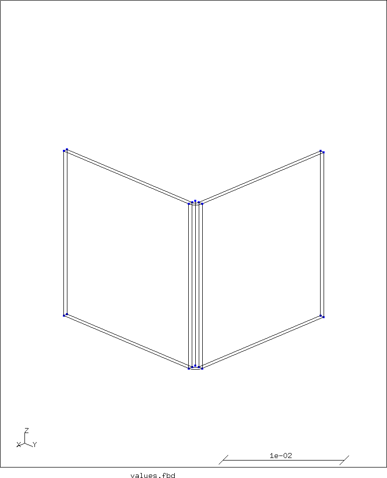
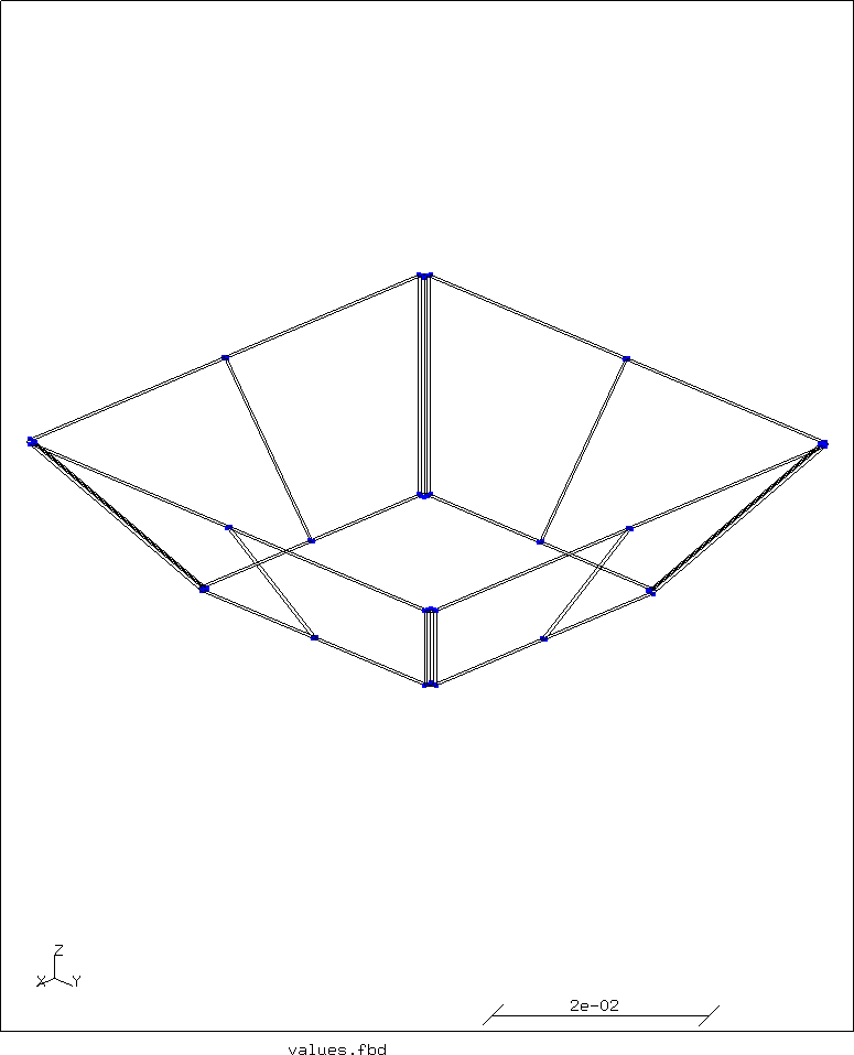
The flexure consists of four folded leaf springs that are connected at the ends to either the fixation or the rigid mody constraint that acts as the load carrying point. See the image of the mesh below.

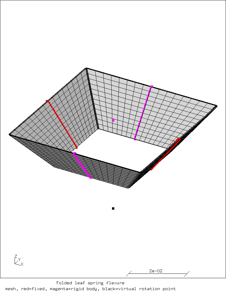
This mesh is a simplified model of a real construction. The red nodes are fixed to the world. In a real construction this would probably be a pair of brackets where the leaf springs are fastened to.

The magenta nodes form the rigid body constraint. The force is applied to the magenta node in the middle. In reality this would be a stiff inverted U-shaped bracket that is connected to the leaf springs.

The black point below the mesh is the virtual point where the fold lines in the leaf springs would meet. This should be the center of rotation.

Creating the geometry and mesh in the preprocessor

The following is the input for the cgx (Calculix GraphiX) preprocessor.

In the preprocessor, points in 3D space can be defined. With those points, lines, arcs and splines can be defined. Lines can then define surfaces, and surfaces can define volumes.

Alternatively, the swep operator can sweep entities into a higher dimensions. So sweeping a point creates a line, sweeping a line creates a surface and sweeping a surface creates a volume. For details, see the cgx manual. That is similar to how modern CAD software creates volumes by extruding a sketch. Sweeping is the technique that will be used here.

First some values are defined and calculated to help with the geometry generation:

## Parameters
# Sizes in [m]
valu X / 30 1000
valu Y X
valu Z / 15 1000
# Wall thickness [m]
valu t / 0.4 1000
# Distance from virtual rotation point to underside [m]
valu ZC / 20 1000
# Height of reference node for rigid body [m]
valu ZR Z
# Number of elements in Y
valu dx2 16
# Number of elements in Z
valu dy2 16
# Twice the number of elements in the radius
valu dr 8
# Twice the number of elements in X
valu dl 24
# Calculated values
valu X2 / X 2
valu Y2 / Y 2
valu X2i - X2 t
valu Y2i - Y2 t
# Number of elements in Y
valu dx2 16
# Number of elements in Z
valu dy2 16
# Twice the number of elements in the radius
valu dr 8
# Twice the number of elements in X
valu dl 24
# Calculated values
valu X2 / X 2
valu Y2 / Y 2
valu X2i - X2 t
valu Y2i - Y2 t
valu Ri t
valu cpx - X2i Ri
valu cpy Y2i
valu ncpx - 0 cpx
valu dx / X2 ZC
valu dx * dx Z
valu dy / Y2 ZC
valu dy * dy Z

Then the geometry is generated.

In step 1 a set is started and point is generated:

seto tube-section
pnt tp1 X2i 0 0

Step 2 takes that point and sweeps it into a line:

swep tube-section new tra t 0 0 4

In step 3, the line is swept into a surface:

swep tube-section ln2 tra 0 cpy 0 dy2

The line at the end of the surface is swept around a point to create a circle section:

pnt cpt cpx cpy 0
swep ln2 ln3 rot cpt z 90 dr

Then the line at the end of that is swept linearly again:

swep ln3 new tra ncpx 0 0 dx2

This whole surface is then extruded:

swep tube-section new tra 0 0 Z dl

Next, the top points are moved outwards in X and Y:

seta points p all
valu t4 * 4 t
enq points pdx rec X2 _  Z t4
enq points pdy rec _  Y2 Z t4
move pdx tra dx 0 0
move pdy tra 0 dy 0

Finally, the whole is mirrored twice to complete the geometry:

copy tube-section new mir y
copy tube-section new mir x
setc
merg p tube-section
merg l tube-section

The geometry is now complete.

Some helper nodes are created and the geometry is meshed with second order quadrilaterally-faced hexahedron elements with reduced integration (he20r):

asgn n 4
node 1 0 0 0
node 2 0 0 ZR
valu nZC - 0 ZC
node 3 0 0 nZC
seta load n 2
seta rotp n 3
elty all he20r
mesh all

The node sets needed to fix the model in space and to act as a rigid body constraint are defined next:

## Fixation and rigid body nodes.
seta nodes n all
enq nodes fix rec _ 0 _ 1e-6
enq nodes rb rec 0 _ _ 1e-6
setr fix n 1 2 3
setr rb n 1 3

Basically, the set fix contains all nodes that have Y-coordinate 0, except nodes 1, 2 and 3. The set rb contains all nodes that have X-coordinate 0, except nodes 1 and 3.

This results in the mesh and extra nodes as shown on the top of this page.

Finally, the nodes, elements and sets are written to disk so the solver can read them in the next step:

## Output data for the solver
send all abq
send fix abq nam
send load abq nam
send rb abq nam
send rotp abq nam

Creating the input for the solver

Now that the mesh has been created we need to define a problem for the solver to calculate. Three different problems will be calculated, with a force acting on the rigid body reference node in X, Y or Z direction. These problems basically only differ in the load vector, so only the first one will be shown.

Finite element programs are basically unitless; it is up to the user to use consistent units. For simplicity, SI units are used both for defining the geometry in the preprocessor and in the solver input file.

A header starts the solver input file:

*HEADING
leaf spring flexure

Next the mesh and named sets are imported:

** Import geometric data
*INCLUDE, INPUT=all.msh
*INCLUDE, INPUT=fix.nam
*INCLUDE, INPUT=load.nam
*INCLUDE, INPUT=rb.nam

The fixation and rigid body constraint are defined:

*RIGID BODY, NSET=Nrb, REF NODE=2
** Fixation
*BOUNDARY
Nfix,1,3

The node set Nrb forms a rigid body. This means that these nodes do not move with respect to each other.

The node set Nfix is fixed in the 1,2 and 3 directions, i.e. X, Y and Z.

At least one material now needs to be defined:

** Material properties
*MATERIAL, NAME=C55S
** werkstoffnr 1.1204
*ELASTIC, TYPE=ISO
190e9,0.29,293
*DENSITY
7820
*EXPANSION, TYPE=ISO
12e-6,293

This is a carbon steel suitable for springs. After forming it is generally hardened and tempered to improve the strength.

Material properties are assigned to the elements. The set Eall contains all elements:

** Apply material properties to element sets.
*SOLID SECTION, ELSET=Eall, MATERIAL=C55S

Finally, a load step is defined. Here, a static analysis with a concentrated load will be used:

*STEP
*STATIC
*CLOAD
2,1,50
*NODE FILE
U,RF
*EL FILE
ZZS,ME
*END STEP

On node 2 (which is part of the rigid body set of nodes), a load of 50 N is applied in the 1 (or X) direction.

For all nodes the displacement (U) and where appliccable the reaction forces (RF) will be recorded in the output file..

For all the elements the stress (ZZS) and strain (ME) will be saved. In the calculation of the stresses the Zienkiewicz-Zhu error estimator is used to improve the accuracy of the stress values at the nodes.

Since this is a relatively small problem with 11678 nodes and 1920 elements, the solver run takes only a couple of seconds on a modern PC.

Results

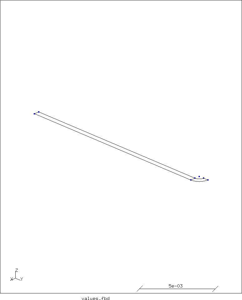
The displacement resulting from the loads in X and Y direction are almost equal. The former is shown below.

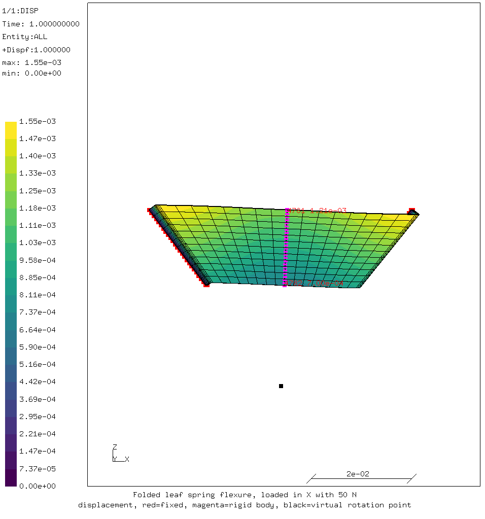
The image clearly shows that the rigid body constraint keeps pointing towards the virtual rotation point at the bottom of the image. The displacement at the top of the rigid body is a lot larger than that at the bottom, as indicated by the numbers in the image.

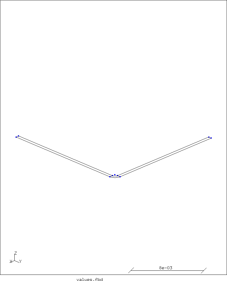
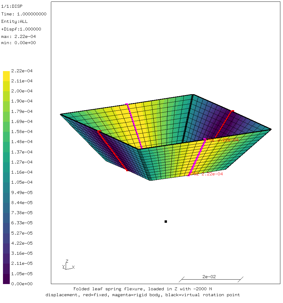
With a much larger load in -Z direction, there is hardly any displacement.