Basics

1. Geometry is generated in a CAD application in the form of a STEP file.
2. The STEP file is batch processed in gmsh using a geo file to produce a mesh and sets for boundary conditions.
3. The mesh is then filtered by a Python script to make it more suitable for use with CalculiX.
4. The analysis is defined in an input file for the CalculiX solver, which includes the mesh, and the analysis is run.
5. Several CalculiX GraphiX scripts are used to show different aspects of the result.

The whole processing is tied together with make.

Generating the STEP file

FreeCAD (using the PartDesign workbench in this case) in is an excellent and free choice to generate solid geometry for analysis.

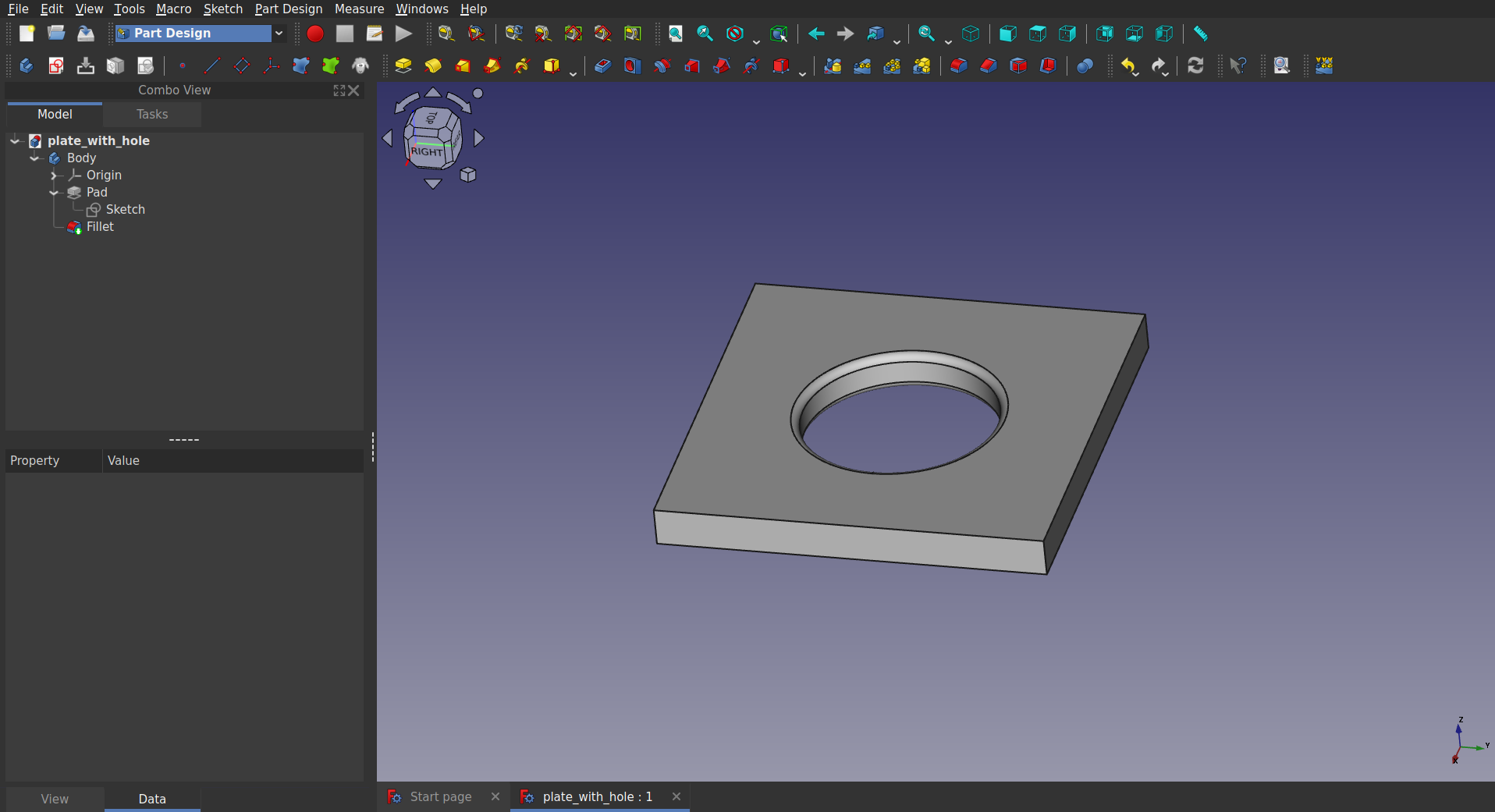
Geometry created in FreeCAD

But whatever CAD program is used, it is important that the geometry is exported as a STEP file defining a solid, or at least a closed shell. If not, meshing might not work.

This STEP file should only contains the features that matter to the analysis. For example small holes and radii in non-critical locations will only serve to increase the size of the mesh and thus the amount of time and memory needed for the analysis. They might even prevent the automatic generation of a functioning mesh. So such features are better suppressed or deleted when generating the STEP file, especially on larger parts. This is a process called “de-featuring”, and is an important part of the workflow.

Here the geometry is a plate of 100×100×10 mm, with a ⌀50 mm hole in the centre. The edges of this hole are rounded. Since this is a simple part, de-featuring is not required here.

Mesh production with gmsh

In general, CAD-generated geometry does not allow for a regular hexahedron-based mesh. But automatic mesh generators are generally able to fill almost any geometry with tetrahedrons.

Initially, the STEP file is opened once in the gmsh GUI, to find the identification numbers of the “Physical Surfaces” that are later used for constraints, see the image below. As long as features are not added to the model, these numbers should be stable. If features are added, the numbering will change and this step should be repeated. With that knowledge, the gmsh input file is written.

To start with, the geometry is imported with the correct units:

SetFactory("OpenCASCADE");
// Convert coordinates to meters
Geometry.OCCTargetUnit = "M";
Merge "plate_with_hole.stp";

To process STEP files, gmsh needs to be compiled with support for the OpenCASCADE geometry kernel. To simplify the FEA, all dimensions are converted to meters so the FEA can be done in SI units.

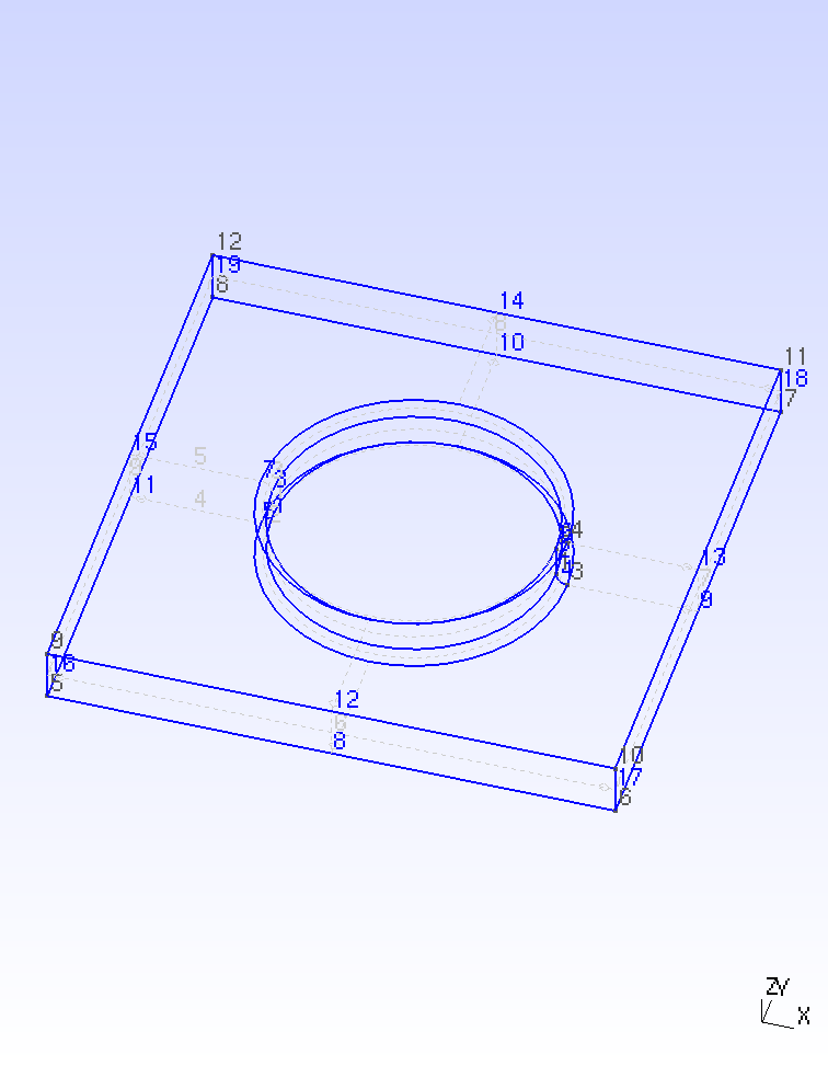
STEP file imported in gmsh with labels visible

Next, physical groups are defined to indicate the which elements and nodes are to be saved. This is based on the surface/volume number that are assigned when the STEP file is merged:

// Describe all physical groups to be saved.
Physical Surface("Nload") = {7};
Physical Surface("Nfix") = {9};
Physical Volume("ignore",1) = {1};

The reason for this is that gmsh creates both a surface mesh and a volume mesh. It is my understanding that the surface mesh is used as a base for creating the volume mesh. But for FEA we’re only interested in the volume mesh. Defining physical groups is a way of not exporting the surface mesh.

Second order elements generally perform better and have fever vices than first order elements. So we make sure to generate second order elements:

Mesh.Algorithm = 2; // Automatic
Mesh.ElementOrder = 2; // Create second order elements.
Mesh.SecondOrderIncomplete = 1;

These settings will generate second order tetrahedral elements.

The following parameters are used to define how fine the mesh should be:

Mesh.MeshSizeFromCurvature = 10;
Mesh.MeshSizeMax = 0.10;
Mesh.Smoothing = 10;

Note that there are several other settings that could also be used. Please consult the gmsh manual.

The Mesh.MeshSizeFromCurvature parameter is used to create more elements at places where the geometry curves. This should create a more accurate image of the stresses at those locations.

Next the mesh is generated and exported:

Mesh.Format = 39; // Save mesh as INP format.
Mesh.SaveGroupsOfNodes = 1;
Mesh.SaveGroupsOfElements = 1;
Mesh.Optimize = 1;
Mesh 3;
OptimizeMesh "Gmsh";
Coherence Mesh;
Save "gmsh-output.inp";

Note that without optimization the mesh might well contain elements with a determinant of the Jacobian matrix < 0. When these occur, gmsh generates a warning. This will inevitably lead to failure of the solver run. Optimizing can often get rid of those. In the cases that it can’t some tweaking of the mesh size generally helps.

If one sets:

Mesh.SaveGroupsOfElements = -1000;

then only volume elements will be exported. If surfaces are not needed, this saves a lot of unnecessary elements.

Processing the mesh

The mesh as generated by gmsh as a CalculiX input file will generally have some traits that are undesirable.

• It will contain a *Heading. This should normally be in the main solver input file.
• Depending on the settings, useless surface elements might be included.
• Volume sets share nodes. This can lead to incorrect stresses.

To fix all this, gmsh-inp-filter is used.

This script performs several actions;

• It removes the *Heading from the mesh file.
• Remaps surface element sets to sets of volume element surfaces.
• Replaces shared nodes between volume sets by equations if needed.
• Writes the improved mesh to a new file.

The script can be called as follows:

python gmsh-inp-filter.py gmsh-output.inp all.msh

The mesh now can be shown in CalculiX GraphiX. The following script (view-mesh.fbd) is used to view the mesh:

# Define the view.
rot y
rot r 15
rot u 30
# Read the mesh.
read all.msh inp
frame
zoom 0.8
# Show the constraints
plus n Nfix b 8
plus f Sload r
# Caption
capt Mesh of 100x100x10 mm EN AW 5754 plate with 50 mm hole
ulin blue = fixed, red = loaded/displaced
# Show the element edges
view elem

This script is called as follows:

cgx -b view-mesh.fbd

This is also a test is the mesh can be read by CalculiX and that the boundary conditions are well-defined. In the following image the finer mesh around the hole is clearly visible.

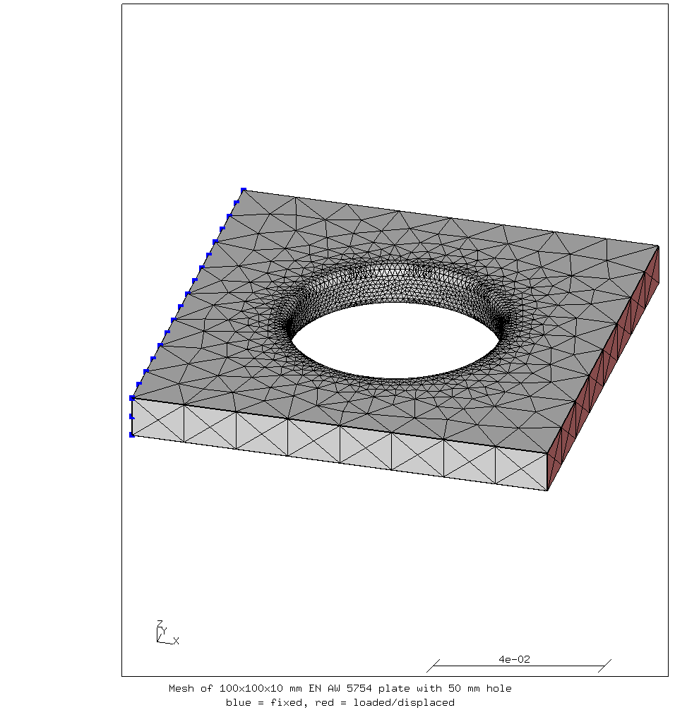
Mesh shown in CalculiX GraphiX

Writing the solver input file and running the analysis

The input file (job.inp) starts with the heading and including the mesh:

*HEADING
plate with hole under tension
*INCLUDE, INPUT=all.msh

Note that all.msh includes the node sets for fixing and loading the part Next the boundary conditions are defined:

*BOUNDARY
Nfix,1,1
** Extra fixation (node in the middle of Nfix) to prevent solid body displacements.
10679,1,3

Now the material properties have to be defined and assigned to the elements. In this case there is only one volume and one material, wrought aluminium alloy EN 5754:

** Material properties
*MATERIAL, NAME=M_EN_AW_5754
*ELASTIC, TYPE=ISO
70e9,0.33,293
*DENSITY
2670
*EXPANSION, TYPE=ISO
23.7e-6,293
** Apply material properties to element sets.
*SOLID SECTION, ELSET=Eall, MATERIAL=M_EN_AW_5754

The yield strength of this material is at least 80 MPa in the H111 temper and can be as high as 180—240 MPa based on the temper. The expected stress is not that high that plastic deformation will be an issue. So it is not necessary to add a *PLASTIC card and define plastic deformation properties here.

Note that if a *PLASTIC card is added to the material definition, the analysis becomes non-linear, and it will take several iterations to finish. In the worst case, the simulation won’t converge, that is the iterations will not get closer and closer to a final answer. Therefore it is advised to start with a linear analysis like this first.

Finally a single load case step is defined:

*STEP
*STATIC
*BOUNDARY
** Prescribed displacement
Nload,1,1,24.31e-6
*NODE FILE
U
*EL FILE
ZZS,ME
** Force in displaced nodes.
*NODE PRINT,NSET=Nload
RF
*END STEP

One should keep in mind that boundary conditions are always approximations and simplifications of the real situation.

In this case, a prescribed displacement is applied to a group of nodes. Especially in case of e.g. material plasticity this will help the solution to converge faster. The displacement was tuned so that the total stress on the load face equals 10 MPa, for a total force of 10 kN.

Alternatively, a rigid body constraint could have been used to apply a force, or a distributed load in the form of a negative pressure could have been applied to the surface.

A rigid body constraint will force all the nodes in the rigid body to have the same displacement, in all directions. This will result in high stresses at the corners of the part that are part of the rigid body. Such stresses are basically an artefact of the rigid body construction, so they can often be ignored; in reality no body is completely rigid.

A distributed load will apply a consistent load, but leaves the displacement free.

The analysis is run, then intermediate files are cleaned up:

ccx -i job
rm -f job.log spooles.out *.12d *.cvg *.sta *Miss*.nam

Using four cores, the analysis takes 3.9 seconds. The results are mainly written to a file job.frd.

Viewing the result

In this section, CalculiX GraphiX will be used to look at the result. The author likes it because it is fast, built-in and can basically show all you need to know to understand the stress situation

But if more “shiny” pictures are required, the results can be post-processed using ccx2paraview to view them in paraview.

Since this is an isotropic material, we will start by viewing the von Mises stress, using the following CalculiX GraphiX script (view-mises.fbd):

rot y
rot r 15
rot u 45

read job.frd
scal d 10
view disp
frame
zoom 0.8

capt 100x100x10 mm EN AW 5754 plate with 50 mm hole
ulin Von Mises stress when loaded with 10 N/mm2 in X-direction

min 0 el
max 50e6 el
cmap viridis
ds 3 e 7
plus nt all r
txt 3036 n
txt 3827 n

It is run as follows:

cgx -b view-mises.fbd

The resulting view is shown below.

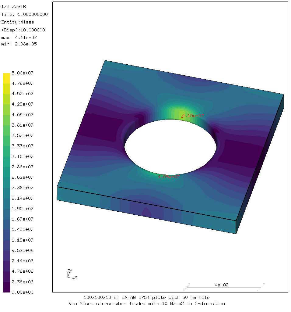
Von Mises stress in the aluminium plate

As expected, there are stress concentrations on the sides of the hole. The average stress next to the hole is 10 kN divided over a surface of 50×10 mm² or 20 MPa. Due to stress concentration around the hole, the real maximum stress is approximately double that. Note that this is still less than the yield strength of the material, so there should be no plastic deformation.

An alternative view is to look at the worst principal stress. In contrast to the von Mises stress, this also shows where the material is in compression. For this the script view-worstps.fbd is used. The bits that are different from the previous viewing script are:

ulin Worst principal stress when loaded with 10 N/mm2 in X-direction

mm 50e6 el
cmap coolwarm
ds 3 e 23
plus nt all k
txt 3036 n
txt 3827 n

In this case the color map and scale is chosen so that tensile stress is red, compressive stress is blue and almost no stress is gray.

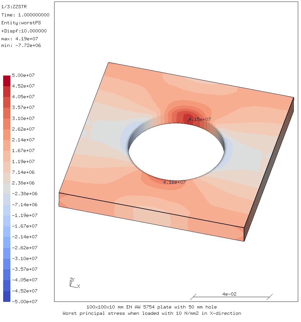
Worst principal stress in the aluminium plate

This image shows that the areas just in front of and just behind the hole are actually in compression and that there are areas without much stress between the hole and the boundaries. This demonstrates that the stress “flows around” the hole, as it were.

Using “make” to automate the analysis

The following Makefile ties all the operations together and enables easy usage.

all: all.msh job.frd

# Run the pre-processor
all.msh: pre.geo gmsh-inp-filter.py
    gmsh pre.geo -
    python gmsh-inp-filter.py gmsh-output.inp all.msh
    rm -f gmsh-output.inp

# Run the solver
# Note: to take advantage of multiple cores,
# OMP_NUM_THREADS should be set in the environment.
job.frd: job.inp all.msh
    ccx -i job
    rm -f job.log spooles.out *.12d *.cvg *.sta
    rm -f *Miss*.nam

# Post-processing commands

mesh: all.msh .PHONY ## view the mesh
    cgx -b view-mesh.fbd

force: job.frd .PHONY ## calculate the load needed for the chosen displacement
    @python force.py job.dat nload x

disp: job.frd view-disp.fbd .PHONY ## view displacements
    cgx -b view-disp.fbd

mises: job.frd view-mises.fbd .PHONY ## view von Mises stress
    cgx -b view-mises.fbd

worstps: job.frd view-worstps.fbd .PHONY ## view worst principal stress
    cgx -b view-worstps.fbd

clean: .PHONY ## clean up the working directory
    rm -f *.equ *.sur *.nam *.msh *.log *.12d *.cvg *.sta *.con
    rm -f spooles.out

help:
    @echo "Command  Meaning"
    @echo "-------  -------"
    @sed -n -e '/##/s/:.*\#\#/\t/p' -e '/@sed/d' Makefile

So if the command make mesh is given from the working directory, the mesh is generated as needed and then displayed. Similarly, make mises shows the von Mises stresses, generating the mesh and running the analysis first if necessary.

The command make help gives an overview of the available commands:

Command  Meaning
-------  -------
mesh     view the mesh
force    calculate the load needed for the chosen displacement
disp     view displacements
mises    view von Mises stress
worstps  view worst principal stress
clean    clean up the working directory