Introduction

In machinery, vibration is generally a fact of life. It is often cost prohibitive and sometimes physically impossible to remove vibrations in use. So any vibration in machinery must be dealt with.

One of the ways of doing that is to make sure that the resonance frequency of parts is higher that the frequencies which are likely to occur. This is especially important for moving parts, where you cannot just massively over dimension them and solidly bolt them down.

The subject of the investigation is a 2 m long tube with a square cross-section and a constant wall thickness over its length. The tube is simply supported at both ends. (This is a mechanical engineering term which basically means that is free to bend but the ends cannot move up and down or sideways.)

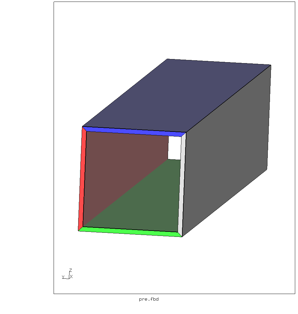
The geometry of one such a tube (W=350, t=15) is shown below. The different colors indicate the four different bodies which are meshed separately. The elements are then connected with tie constraints.

The variables in this investigation are the outside width and height of the tube, the wall thickness and the laminate lay-up.

For calculating the resonance frequencies of a tube the CalculiX (alternate link) finite element analysis software is used.

Calculation

The CalculiX software consists of two programs.

• The preprocessor creates the geometry and mesh. It also can display the results.
• The solver takes a well-defined field problem and solves it.

Both the pre- and post processor (cgx) and the solver (ccx) are driven by plain-text input files, which makes it rather easy to automate.

The outside size of the beam will be varied between 100 mm and 350 mm in steps of 50 mm. The wall thickness is varied in steps of 1 mm, with the minimum and maximum thickness depending on the outside size. The size and wall thickness are defined in the preprocessor file (pre.fbd) to generate the required geometry and mesh.

A Python script has been used to automate the whole thing. For each combination of size and wall thickness it does the following:

• Update the preprocessor file pre.fbd with the correct dimensions.
• Run the preprocessor cgx to create the mesh.
• Run the solver.
• Extract the first resonance frequency from the results file.
• Print a line containing size, wall thickness and first resonance frequency.

When the script is run, the output is redirected to a text file. The full source code (with comments) is shown below.

import os
import subprocess as sp

# Save the return status of preprocessor and solver.
error = 0
# Environment setting for the solver to use multiple cores.
ccxenv = os.environ
ccxenv["OMP_NUM_THREADS"] = "4"

variables = [
   # width, tmin, tmax
   (100, 1, 6),
   (150, 2, 5),
   (200, 5, 14),
   (250, 7, 17),
   (300, 9, 19),
   (350, 10, 20),
]

os.chdir("berekeningen")
for W, tmin, tmax in variables:
   for T in range(tmin, tmax + 1):
      # Bail out if an error has occurred.
      if error:
            os.chdir("..")
            exit(1)
      # Edit the dimensions in the preprocessor file.
      with open("pre.fbd", "r") as pre:
            prelines = pre.readlines()
      prelines[0] = f"valu W / {W} 1000{os.linesep}"
      prelines[1] = f"valu T / {T} 1000{os.linesep}"
      with open("pre.fbd", "w") as pre:
            pre.writelines(prelines)
      # Run the preprocessor and check for errors.
      cgx = sp.run(["cgx", "-bg", "pre.fbd"], stdout=sp.DEVNULL, stderr=sp.DEVNULL)
      if cgx.returncode != 0:
            error = cgx.returncode
            break
      # Merge all tie constraints into a single file.
      sp.run(
            "cat DCF* ICF* >ties.sur",
            shell=True,
            stdout=sp.DEVNULL,
            stderr=sp.DEVNULL,
      )
      sp.run(
            "rm -f DCF* ICF*",
            shell=True,
            stdout=sp.DEVNULL,
            stderr=sp.DEVNULL,
      )
      # Run the solver and check for errors.
      ccx = sp.run(
            ["ccx", "-i", "job"],
            env=ccxenv,
            stdout=sp.DEVNULL,
            stderr=sp.DEVNULL,
      )
      if ccx.returncode != 0:
            error = ccx.returncode
      # Clean up generated files.
      sp.run(
            "rm -f job.log spooles.out *.12d *.cvg *.sta *Miss*.nam",
            shell=True,
            stdout=sp.DEVNULL,
            stderr=sp.DEVNULL,
      )
      # Extract the resonance frequency.
      with open("job.dat") as datfile:
            dat = datfile.readlines()
      freq = float(dat[7].split()[3])
      # Write the output for this iteration.
      print(f"{W} {T:2d} {round(freq, 2):.2f}", flush=True)
   # Add a blank line after each group of the same outside dimension.
   print()

Each run of this script produced a file with around 60 FEA results. Doing that all by hand would be tedious and error-prone. So automating it was very much worth the effort.

Between runs I’ve edited the solver input file to assign different material properties to the elements. This was so the influence of different laminate stack-ups can be shown. In total I had around 240 resulting tuples of (width, height, resonance frequency). From the width, thickness, length and the density of the material, the weight of the beam can also be calculated.

Results

Looking at the individual results, I could basically see two different types of response.

What one would expect is a global deformation of the beam, which is what is shown below on the left.

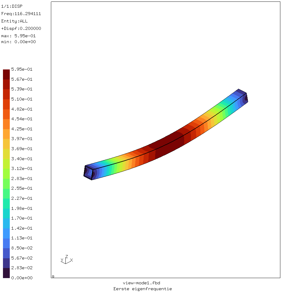
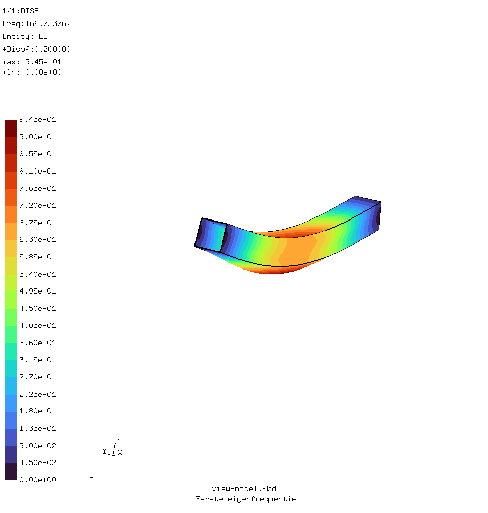
With some of the geometries, significant deflection of the faces that make up the beam could be seen. This is shown in the right image above. This tends to occur when the faces are relatively thin compared to the width of the beam. These geometries tend to have lower eigenfrequencies.

For this kind of beam, torsion does not seem to be an expected first eigen mode.

Presentation

Now I had to decide how best to visualise all the results. Basically this is a four-dimensional data set, which is not easily shown on the two-dimensional space of a piece of paper or screen.

The data set has two input variables; width, (height) and wall thickness. There are also two output variables: first eigenfrequency and weight of the beam.

So I decided to do a 2×2 grid of plots, with the input variables on the x-axes, and output on the y-axes. This grid is shown below.

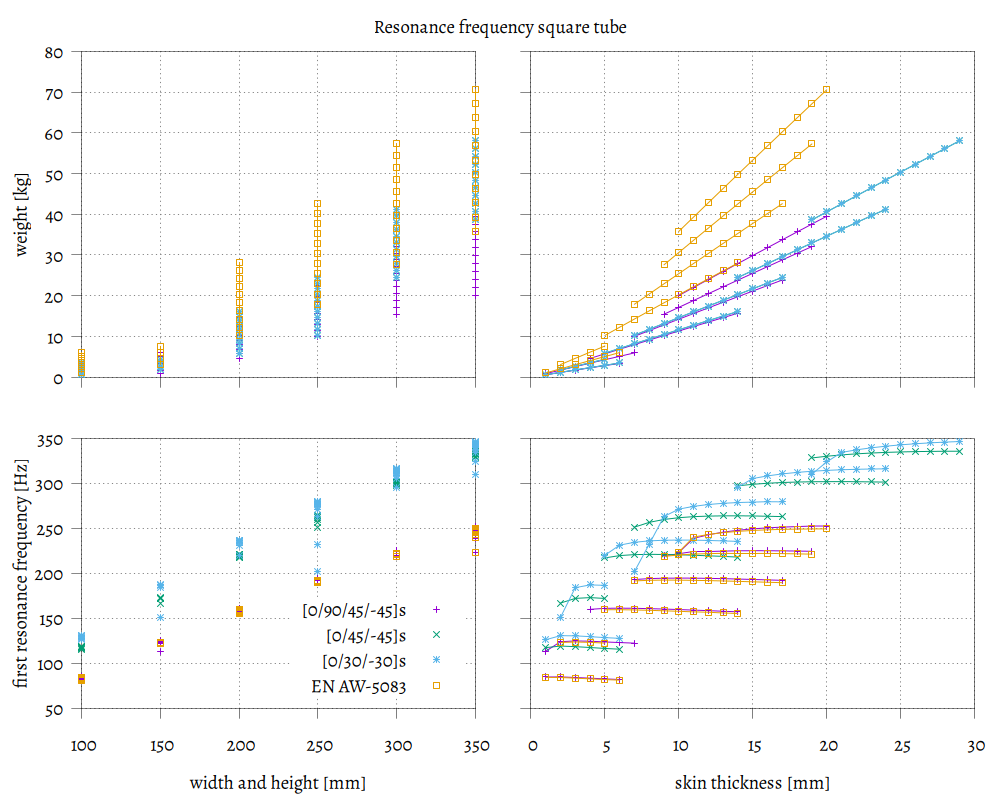
So what can we learn from these figures?

From the figure on the bottom left we see that: (1) The first eigenfrequency tends to go up with the width and height. Initially I thought this was a linear gain, but it does tend to taper off for higher widths.

The quasi isotropic laminate performs about as well as the aluminium. (2) For the same width and height, more specialized laminates perform *significantly* better.

Looking at the bottom right picture we can see that for very thin walls the eigenfrequency tends to drop off. This corresponds with the vibrations of the walls as shown above. (3) Once you reach a certain thickness sufficient for wall stability, any more wall thickness is only a marginal improvement.

However, with larger beam sizes the minimum required wall thickness increases faster. Looking at the right top figure we can see that: (4) adding extra wall thickness adds weight (and thus cost) faster than it does eigenfrequency, once the walls are thick enough not to wobble.

The weight graph could have been improved by converting it into a material cost graph. This could be done by multiplying the weight by the price/kg if the different materials. This would account for the reality that carbon/epoxy laminate is much more expensive on a per kg basis than aluminium.