Using the pre-processor to generate the mesh

Since this situation is symmetrical, we will only simulate half of it (C−B). When showing the results they will be mirrored to show the whole beam. And instead of moving point C downwards, we will move point B upwards. That amounts to the same deformation in the sandwich, just with another reference point.

For simplicity, we will apply constraints and displacements directly to the nodes. In reality, the beam usually rests on cylindrical supports, but that is for a later article.

We will use the domain-specific language (“DSL”) of the CalculiX pre-processor cgx to generate the geometry. We start with defining the parameters for the model.

# Dimensions:
#  length in m of half the sample
valu L / 0.56 2
# detailed length
valu D / L 10
valu D2 * D 2
valu Lp3 - L D2
# width in m
valu B 0.1
valu B2 / B 2
# total thickness in m
valu T 0.031
# top skin thickness in m.
valu t1 0.0015
# bottom skin thickness in m.
valu t2 0.0015
# core thickness in m
valu tk - T t1
valu tk - tk t2

# Divisions that determine element count.
# Note that for second order elements, two divisions is one elemen!
# divisions in length.
valu ldiv 40
# divisions in length.
valu ddiv 10
# devisions in width.
valu bdiv 12
# divisions in skin height.
valu tbdiv 6
# divisions in core height
valu tkdiv 6

Next we create the volumes.

# Bottom skin
seto skin2
    pnt ! 0 0 0
    swep skin2 p2 tra D 0 0 ddiv
    swep p2 p3 tra Lp3 0 0 ldiv
    swep p3 new tra D 0 0 ddiv
    swep skin2 new tra 0 B 0 bdiv
    swep skin2 if1 tra 0 0 t2 tbdiv
setc
# Core
seto core
    copy if1 if2 tra 0 0 0
    swep if2 if3 tra 0 0 tk tkdiv
setc
# Top skin
seto skin1
    copy if3 if4 tra 0 0 0
    swep if4 top tra 0 0 t1 tbdiv
setc

Note that in the length the model is divided into three parts. The reason for that is that we want the mesh to be finer near the points where the load and displacement constraints are applied because that is where the stress concentrations will be.

Generally, one would want the mesh near a stress concentration fine enough that the effects of the stress concentration are spread of several elements. Otherwise the way the element is defined (the shape functions) will determine how the stress concentration looks.

Next, we can create the mesh, create the node sets for the constraints. In this case for this simple sandwich we will use equations to tie the different materials together.

See part 1 on why we want to do this instead of just make the elements from different materials share nodes.

# Constraints
seta nodes n all
enq nodes fix rec 0 _ T 0.0001 a
enq nodes symm rec 0 _ _ 0.001 a
setr symm n fix
enq nodes disp rec L _ 0 0.0001 a
# Write contact equations
send if1 if2 abq areampc 123
send if3 if4 abq areampc 123
# Remove nodes on dependant contact surfaces from constraints
setr fix n if1 if3
setr symm n if1 if3

The CalculiX manual recommends using tie constraints, but equations also work. The potential problem with using equations is that a node can only appear on the dependant side of an equation once, otherwise the solver run will fail. This can be hard to do with the pre-processor on complex parts, and tie constraints do not have that problem.

The last pre-processing step involves writing the data.

# Write data
send all abq
send skin2 abq nam
send core abq nam
send skin1 abq nam
send fix abq nam
send symm abq nam
send disp abq nam
quit

Using the quit command enables us to use the -bg option of cgx. This suppresses the graphics output for the creation of the mesh. The finished mesh is shown below.

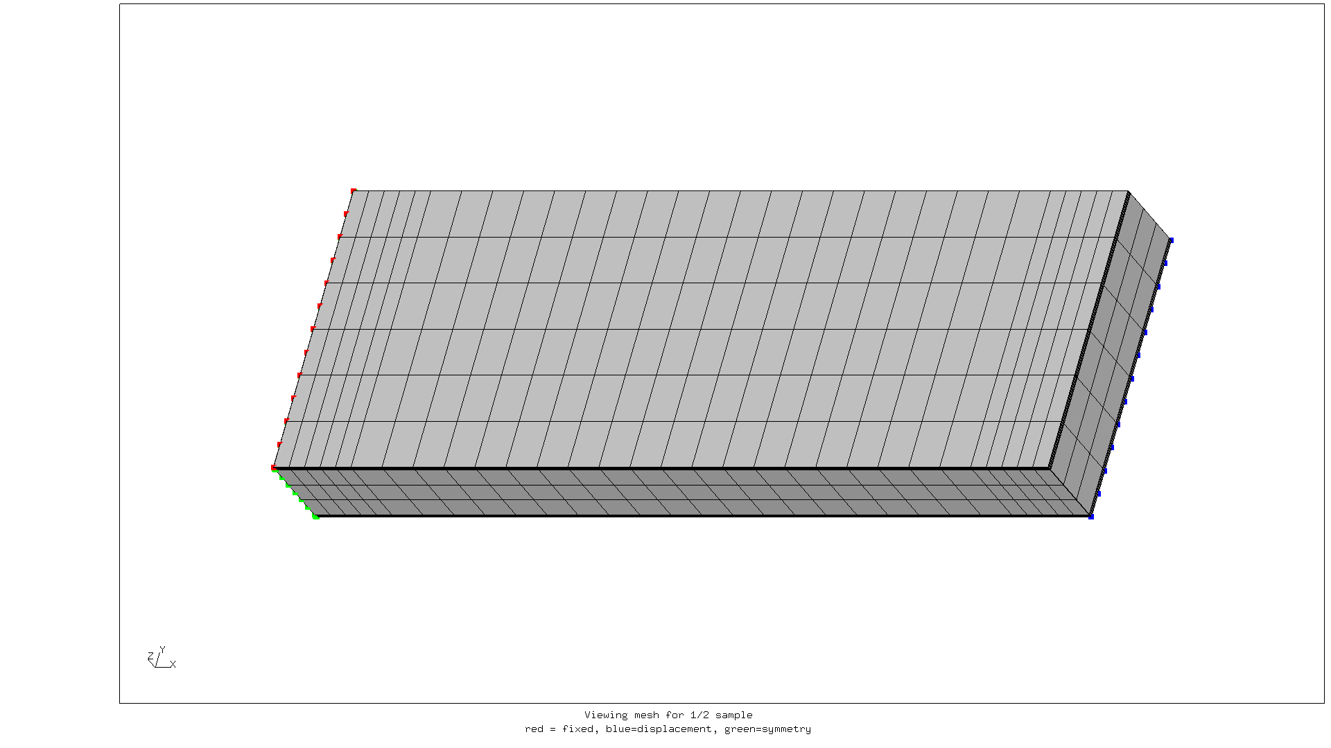
One can see how the mesh size is smaller near the ends. The red nodes will be fixed in all directions. The green nodes will be fixed in x-direction. The blue nodes will be subject to a forced displacement.

Writing the solver command file

First we need to import all the files generated by the preprocessor.

*HEADING
Three-point bending of sandwich
** Import geometry
*INCLUDE, INPUT=all.msh
*INCLUDE, INPUT=core.nam
*INCLUDE, INPUT=disp.nam
*INCLUDE, INPUT=fix.nam
*INCLUDE, INPUT=if1.equ
*INCLUDE, INPUT=if3.equ
*INCLUDE, INPUT=skin1.nam
*INCLUDE, INPUT=skin2.nam
*INCLUDE, INPUT=symm.nam

Then we apply the boundary conditions.

** Fix the middle of the beam.
*BOUNDARY
Nfix,1,3
Nsymm,1,1

Next come the material definitions. This sandwich consists of a Rohacell 71IG core, with a stainless steel (1.4301) skin on top and an aluminium (EN AW-5083) skin on the bottom.

In tests like these, materials are generally tested until failure or permanent deformation occurs. So we have to take plastic deformation into account. Metals are well-known to exhibit plastic behavior. We have used the Ramberg-Osgood equation to generate the plastic deformation curve for the metal skins.

The metal materials are defined as follows.

** Steel
*MATERIAL, NAME=M1.4301
*ELASTIC, TYPE=ISO
200e9,0.30,293
*PLASTIC, HARDENING=COMBINED
205e6,0.003025,293
300e6,0.019373,293
400e6,0.095501,293
475e6,0.253618,293
515e6,0.402575,293
*DENSITY
7900

** Aluminium
*MATERIAL, NAME=M_EN_AW_5083
*ELASTIC, TYPE=ISO
71e9,0.33,293
** H111: Rp = 150, Rm = 310, em = 0.13
*PLASTIC, HARDENING=COMBINED
150e6,0.002,293
175e6,0.00485,293
200e6,0.01046,293
250e6,0.03773,293
280e6,0.0724,293
*DENSITY
2660

For the core foam I decided to use the datasheet properties for compression, since in this case the foam will definitely experience it next to shear. The plastic properties are estimated from a compression test, where the force showed practically no increase after cells started failing.

*MATERIAL, NAME=MrohacellIG71
*ELASTIC,TYPE=ENGINEERING CONSTANTS
73e6,73e6,73e6,0.1,0.1,0.1,29e6,29e6
29e6,293
*PLASTIC
** This is a guess.
1.5e6,0.0,293
1.5e6,0.1,293
*DENSITY
75

As usual, we have to assign materials to the different element sets.

*SOLID SECTION, ELSET=Eskin2, MATERIAL=M_EN_AW_5083
*SOLID SECTION, ELSET=Ecore, MATERIAL=MrohacellIG71
*SOLID SECTION, ELSET=Eskin1, MATERIAL=M1.4301

Here is the *STEP section. It is somewhat different from the earlier examples.

*STEP, NLGEOM
*STATIC
*BOUNDARY
** Forced displacement 10 mm
Ndisp,3,3,10e-3
*NODE FILE
U
*NODE PRINT,NSET=Ndisp
RF
*EL FILE
ZZS,PEEQ
*END STEP

We use the NLGEOM option to tell the solver that nonlinear geometric effects are to be taken into account. As a consequence, this will become an iterative calculation.

Inside the step, the *BOUNDARY command is used to enact the forced displacement.

The *NODE PRINT command is used to save the reaction force on the nodes in the set Ndisp in a .dat file for later use.

Finally, for the elements we not only save the Zienkiewicz-Zhu improved stress (ZZS), but also equivalent plastic strain (PEEQ).

Results

The solver run took around 27 seconds on my i7-7700 class machine. Maximum resident set size was about 0.5 GiB. The solver divided the total displacement into four steps, which each took four to five iterations for the calculations to converge.

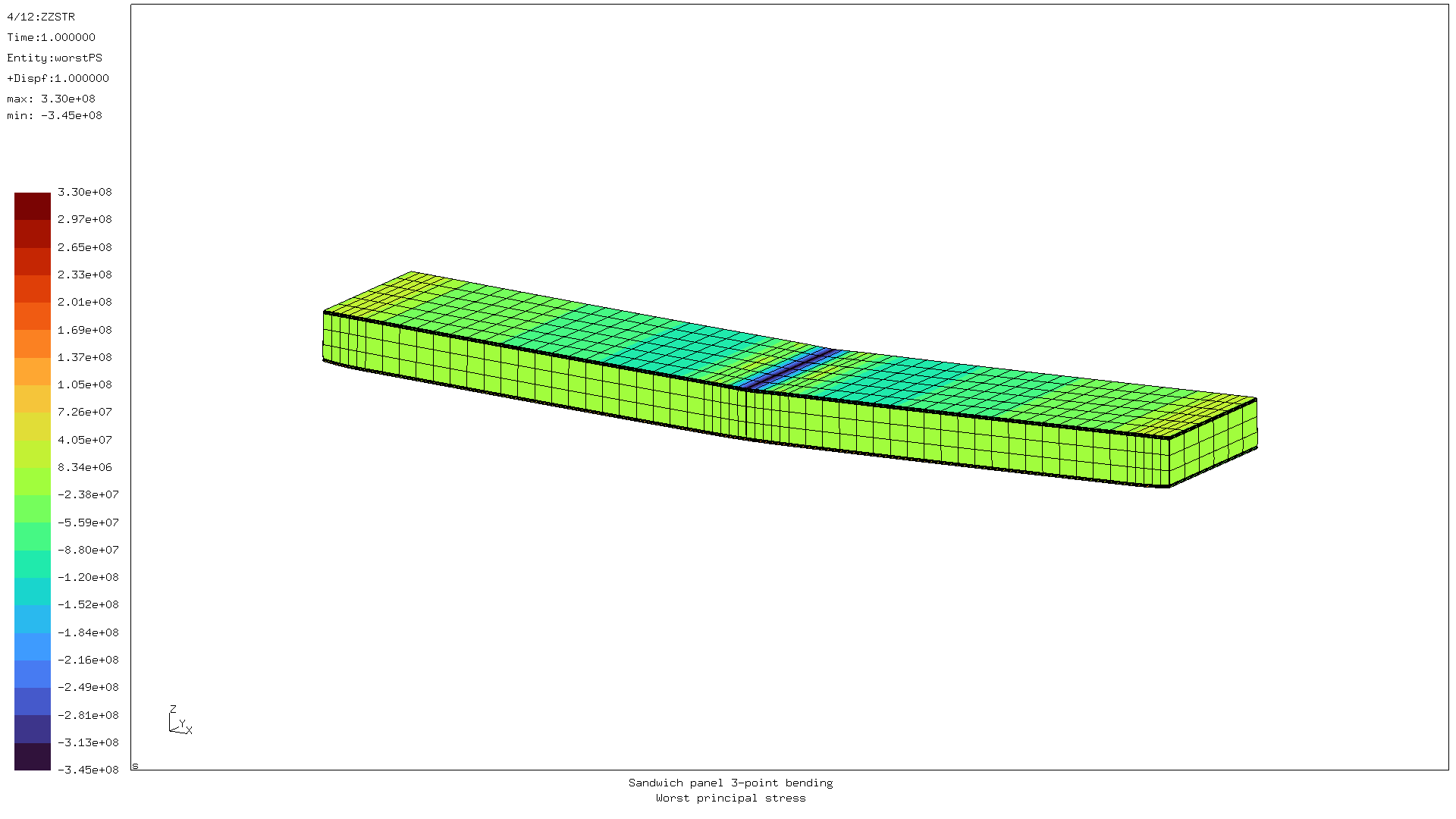
It is clear that the largest compression occurs in the middle of the top skin, as expected. So let’s look at the stress in the skins in more detail.

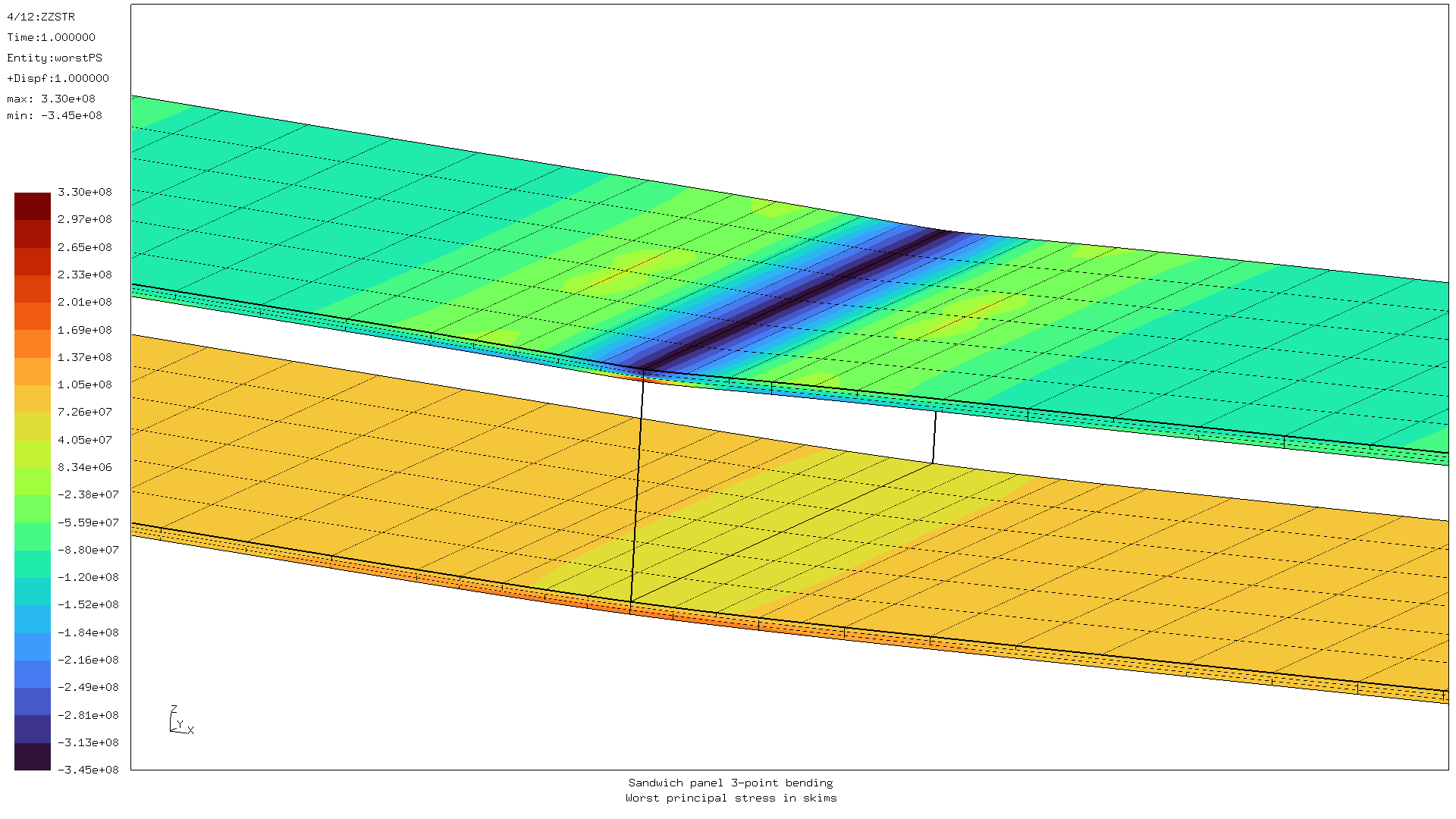
If we look at the side of the top skin we can see that the maximum tension stress also occurs in the top skin, but on its bottom side. This is confirmed if we look at the plastic strain.

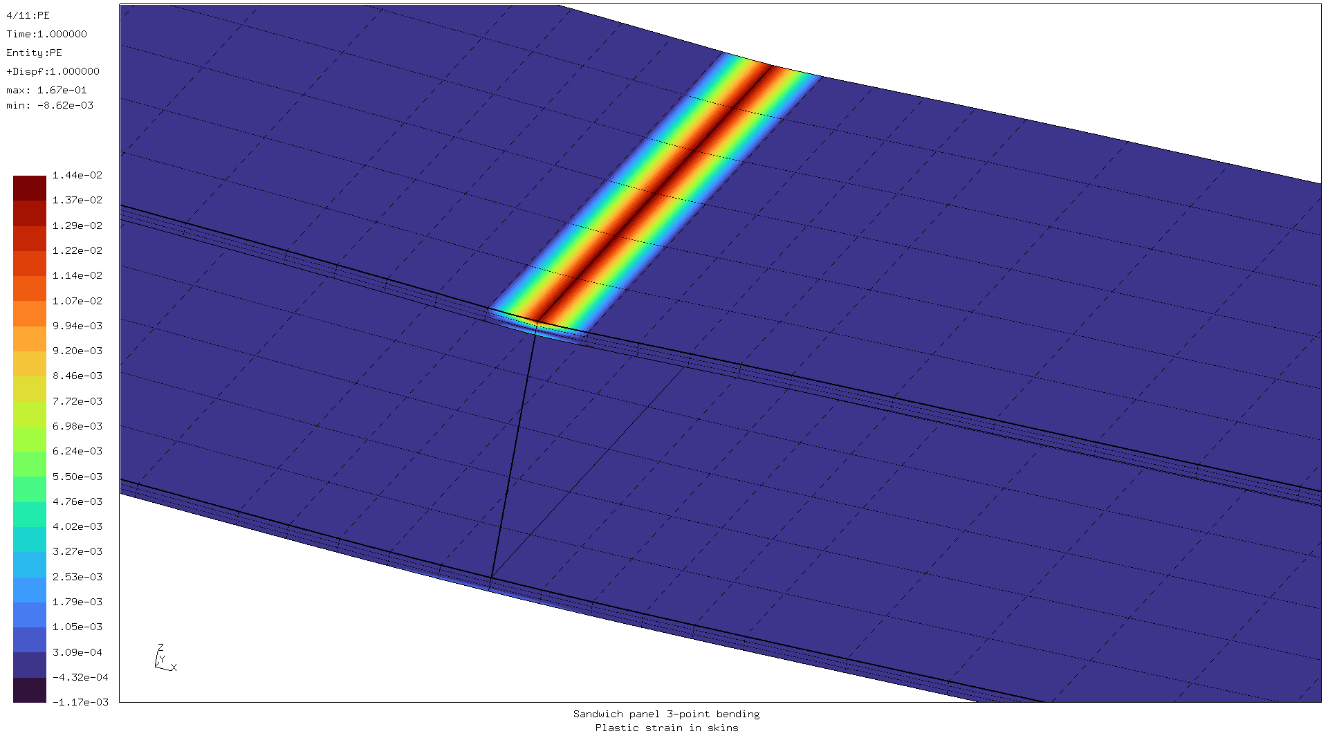
The top skin in the middle of the beam is the place where the highest plastic strain occurs in the skin.

The reaction force data for each step is saved in text format in a .dat file (first two steps shown):

forces (fx,fy,fz) for set NDISP and time  0.2500000E+00

    2599 -3.360807E-06 -4.033513E-07  2.057916E+01
    2600 -9.987526E-06  8.358038E-07  3.045198E+01
    2607  3.979269E-05 -1.930124E-07  5.925281E+01
    2729 -8.014658E-06 -9.461500E-08  2.950608E+01
    2733  3.352114E-05  2.411522E-07  6.555898E+01
    2804 -7.927693E-06 -2.026624E-10  2.993997E+01
    2808  3.389915E-05  7.729466E-08  6.561188E+01
    2879 -8.013995E-06  9.449739E-08  2.950608E+01
    2883  3.389901E-05 -7.687667E-08  6.561188E+01
    2954 -9.987691E-06 -8.355860E-07  3.045198E+01
    2958  3.352070E-05 -2.414209E-07  6.555898E+01
    3029 -3.360673E-06  4.033751E-07  2.057916E+01
    3033  3.979238E-05  1.928583E-07  5.925281E+01

forces (fx,fy,fz) for set NDISP and time  0.5000000E+00

    2599  4.537729E-08 -4.412250E-09  4.159682E+01
    2600  1.061603E-07 -1.883946E-09  6.000885E+01
    2607 -2.892327E-07  2.667418E-09  1.151232E+02
    2729  8.682119E-08 -3.611315E-10  5.755900E+01
    2733 -2.277925E-07  4.297348E-10  1.300878E+02
    2804  8.640352E-08  6.263113E-11  5.837196E+01
    2808 -2.253813E-07  1.549903E-10  1.302890E+02
    2879  8.613001E-08  2.752583E-10  5.755900E+01
    2883 -2.249354E-07 -4.085367E-10  1.302890E+02
    2954  1.058637E-07  1.811355E-09  6.000885E+01
    2958 -2.271329E-07 -3.161963E-10  1.300878E+02
    3029  4.525147E-08  4.314001E-09  4.159682E+01
    3033 -2.885772E-07 -2.396299E-09  1.151232E+02

To make a force/displacement graph for this simulation, a small Python script was used to sum the z-forces per step.

disp = 0
zf = 0
print("0.0000 0")
with open("static.dat") as f:
    for ln in f:
        ln = ln.strip()
        if ln.startswith("forces"):
            if zf:
                print(f"{disp:.4f} {zf:.0f}")
            zf = 0
            disp = float(ln.split()[-1])*0.01  # m
            pass
        elif len(ln) > 0:
            zf += 2*float(ln.split()[-1])
print(f"{disp:.4f} {zf:.0f}")

The resulting data was turned into a plot with gnuplot.

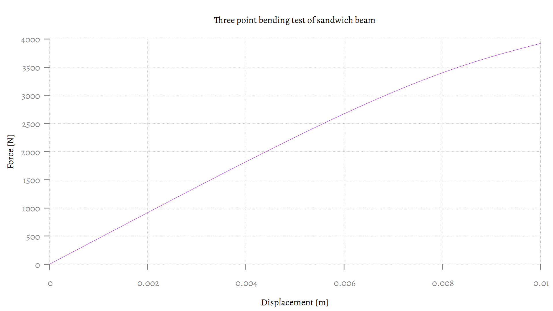
This graph was a good match when actual samples were subjected to the three point bending test.